Stacked Generalization for Materials Property Prediction: A Comprehensive Framework for Accelerated Discovery
This article provides a comprehensive exploration of stacked generalization, an advanced ensemble learning technique, for predicting materials properties.
Stacked Generalization for Materials Property Prediction: A Comprehensive Framework for Accelerated Discovery
Abstract
This article provides a comprehensive exploration of stacked generalization, an advanced ensemble learning technique, for predicting materials properties. Tailored for researchers, scientists, and drug development professionals, it details the foundational theory of stacking, its methodological implementation using diverse base learners and meta-models, and strategies for troubleshooting common challenges like computational cost and data scarcity. Through validation against individual models and other advanced frameworks, the article demonstrates the superior accuracy and robustness of stacking for applications ranging from high-entropy alloy design to molecular property prediction in drug discovery. The synthesis offers practical insights for integrating this powerful AI tool into materials development pipelines to enhance efficiency and predictive performance.
The Foundation of Stacked Generalization: From Basic Theory to Materials Science Applications
In the rapidly evolving field of materials science, accurately predicting properties such as the yield strength of high-entropy alloys (HEAs) or the compressive strength of sustainable concrete is paramount for accelerating the discovery and development of next-generation materials [1] [2]. Traditional experimental approaches and single-model computational methods often struggle with the vast compositional space and complex, non-linear interactions inherent in these material systems. Ensemble learning has emerged as a powerful machine learning paradigm that addresses these challenges by combining multiple models to achieve superior predictive performance and robustness compared to any single constituent model [3] [4]. This article provides a detailed introduction to the three cornerstone ensemble techniques—Bagging, Boosting, and Stacking—framed within the context of advanced materials property prediction. We will delineate their core mechanisms, illustrate their applications with quantitative comparisons, and provide detailed experimental protocols for their implementation in research settings, with a special emphasis on stacked generalization.
Core Ensemble Methods: Mechanisms and Comparisons
Bagging (Bootstrap Aggregating)
Bagging is designed primarily to reduce variance and prevent overfitting, especially in high-variance models like deep decision trees [4].
- Mechanism: It creates multiple bootstrap samples (random subsets with replacement) from the original training dataset. A base model, often referred to as a base learner, is trained independently on each of these samples. During prediction, for regression tasks, the outputs of all models are averaged; for classification, a majority vote is taken [4].
- Key Advantage: The independence of base model training allows for parallel processing, significantly reducing computation time [4].
- Representative Algorithm: Random Forest is an extension of bagging that further de-correlates trees by randomly selecting a subset of features at each split, enhancing model robustness [4].
Boosting
Boosting is a sequential ensemble method that focuses on reducing bias by iteratively learning from the errors of previous models [4].
- Mechanism: It trains a sequence of weak learners, where each subsequent model pays more attention to the training instances that were misclassified by its predecessors. This is typically achieved by adjusting the weights of data points. The final prediction is a weighted sum of the predictions from all weak learners [4].
- Key Advantage: Boosting often leads to high predictive accuracy and is particularly effective on structured or tabular data [4].
- Representative Algorithms: AdaBoost (Adaptive Boosting) and Gradient Boosting, including its advanced implementations like XGBoost and LightGBM [5] [4].
Stacking (Stacked Generalization)
Stacking is a more advanced ensemble technique that introduces a hierarchical structure to combine multiple, potentially diverse, base models using a meta-learner [1] [4].
- Mechanism: The process involves two levels. At Level-0, diverse base models (e.g., Random Forest, Gradient Boosting, Support Vector Machines) are trained on the original data. Their predictions on a validation set (often generated via cross-validation) form a new dataset, known as the meta-features. At Level-1, a meta-model (or meta-learner) is trained on these meta-features to learn the optimal way to combine the predictions of the base models [1] [4].
- Key Advantage: Stacking leverages the strengths of different algorithmic approaches, often capturing complex patterns that a single model type might miss, thereby frequently achieving state-of-the-art predictive performance [1] [6].
- Application Context: It has been successfully applied in diverse prediction tasks, from the yield strength of high-entropy alloys [1] to automated real estate valuation [7] [6].
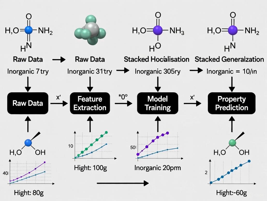
The following workflow diagram illustrates the structured process of a stacking ensemble, from data preparation to final prediction.
Quantitative Performance Comparison
The table below summarizes a comparative analysis of the three ensemble methods, synthesizing performance metrics reported across various applied studies in materials science and property valuation.
Table 1: Comparative Analysis of Ensemble Learning Methods
| Ensemble Method | Reported Performance Metrics | Key Advantages | Common Applications |
|---|---|---|---|
| Bagging (e.g., Random Forest) | High feature importance interpretability; Effective variance reduction [4]. | Parallelizable training, robust to noise and overfitting [4]. | Phase classification in HEAs [1], concrete strength prediction [2]. |
| Boosting (e.g., XGBoost, LightGBM) | Often the top-performing base model; LightGBM: AUC=0.953, F1=0.950 [5]; XGBoost: R²=0.983 for concrete strength [2]. | High predictive accuracy, effective bias reduction [4]. | Predicting student academic performance [5], strength of concrete with industrial waste [2]. |
| Stacking | Marginal but significant improvement over best base model; MdAPE reduction from 5.24% (XGB) to 5.17% [7]. | Leverages model diversity, often achieves state-of-the-art results [1] [6]. | HEA mechanical property prediction [1], automated valuation models (AVMs) [7] [6]. |
Experimental Protocol for Stacked Generalization
This protocol provides a step-by-step guide for developing a stacking ensemble model, tailored for predicting materials properties such as the yield strength of High-Entropy Alloys (HEAs) [1].
Dataset Preparation and Feature Engineering
- Data Collection: Compile a dataset from publicly available materials databases and literature. For HEA prediction, the dataset should include composition, processing conditions, and measured mechanical properties [1].
- Feature Pooling: Extract key physicochemical features and derived parameters. These may include atomic radius, electronegativity, valence electron concentration, and mixing enthalpy [1].
- Feature Selection: Implement a feature selection strategy to identify the most relevant descriptors. The Hierarchical Clustering-Model-Driven Hybrid Feature Selection (HC-MDHFS) strategy can be employed:
- Use hierarchical clustering to group highly correlated features, reducing redundancy.
- Dynamically select the best feature subset based on the performance of base learners [1].
- Data Splitting: Split the dataset into training (e.g., 75%) and testing (e.g., 25%) sets. Ensure the splits are representative and, if necessary, stratified [7].
Model Training and Validation: Level-0
- Base Learner Selection: Choose diverse, high-performing algorithms as base models. Recommended models include:
- Cross-Validation for Meta-Features:
- Perform k-fold cross-validation (e.g., 5-fold) on the training set for each base model.
- For each model and each fold, retain the out-of-fold predictions on the validation folds. Concatenating these predictions forms a new feature set, the meta-features, which serve as the training data for the meta-learner [4].
- Optionally, make predictions on the hold-out test set using the full base models trained on the entire training set. These will be the test-set meta-features.
Model Training and Validation: Level-1
- Meta-Learner Selection: Train a meta-model on the meta-features dataset. Simpler, linear models are often effective to prevent overfitting.
- Final Model Training: The final stacking model is an integrated pipeline of the base learners and the meta-learner.
Model Interpretation and Validation
- Performance Evaluation: Validate the final stacked model on the held-out test set using metrics relevant to the field: Root Mean Squared Error (RMSE), Coefficient of Determination (R²), and Median Absolute Percentage Error (MdAPE) [1] [7] [2].
- Interpretability Analysis: Apply model interpretation techniques like SHapley Additive exPlanations (SHAP) to assess the global and local importance of features in the model's predictions, providing insights into the underlying physical factors governing material properties [1] [5].
The Scientist's Toolkit: Essential Research Reagents & Solutions
The following table details key computational and methodological "reagents" required for implementing ensemble models in materials informatics research.
Table 2: Key Research Reagents and Computational Tools for Ensemble Learning
| Item Name | Function / Application | Example / Specification |
|---|---|---|
| Scikit-learn | A core Python library providing implementations of Bagging, Boosting (AdaBoost, Gradient Boosting), and Stacking classifiers/regressors, along with data preprocessing and model selection tools [4]. | sklearn.ensemble.StackingClassifier |
| XGBoost / LightGBM | Optimized gradient boosting libraries designed for speed and performance, frequently serving as high-performance base learners in ensembles [5] [2]. | xgb.XGBRegressor() |
| SHAP (SHapley Additive exPlanations) | A unified framework for interpreting model predictions, crucial for explaining complex ensemble models and deriving scientific insights from materials informatics models [1] [5]. | shap.TreeExplainer() |
| Molecular Embedders | Algorithms that transform molecular or crystal structures into numerical vectors (descriptors), enabling the application of ML to chemical and materials data [8]. | VICGAE, Mol2Vec [8] |
| HC-MDHFS Strategy | A hybrid feature selection method that uses hierarchical clustering to reduce multicollinearity before a model-driven selection of the most predictive features for the target property [1]. | Custom implementation based on domain knowledge and model feedback. |
| Synthetic Minority Oversampling (SMOTE) | A data balancing technique used to address class imbalance in datasets, which can be critical for predictive tasks involving rare phases or failure modes [5]. | imblearn.over_sampling.SMOTE |
Stacked generalization, or stacking, is an advanced ensemble machine learning technique designed to enhance predictive performance by combining multiple models. Its core principle involves a two-layer architecture: a set of base learners (level-0 models) that make initial predictions from the original data, and a meta-learner (level-1 model) that learns to optimally combine these predictions to produce a final output [9]. This approach is particularly valuable in materials science and drug development, where it can uncover complex relationships between processing parameters, chemical compositions, and functional properties, thereby accelerating the discovery of new materials and compounds [10] [11].
Core Architectural Principles
The architecture of stacked generalization is fundamentally designed to leverage the strengths of diverse modeling approaches.
The Base Learner Layer
Base learners are a set of heterogeneous models trained independently on the same dataset. Their purpose is to capture different patterns or perspectives within the data. Diversity among base models is critical; using models with different inductive biases (e.g., tree-based methods, linear models, neural networks) ensures that the meta-learner receives a rich set of predictive features. This diversity reduces the risk of the ensemble inheriting the limitations of any single model [7] [9].
The Meta-Learner Layer
The meta-learner is a model trained on the outputs of the base learners. Its input is the vector of predictions made by each base model, and its objective is to learn the most effective way to combine them. For example, it might learn to trust one model for certain types of inputs and another model for different scenarios. Common choices for meta-learners include linear models, logistic regression, or other algorithms that can effectively model the relationship between the base predictions and the true target [12] [13]. The success of stacking hinges on the meta-learner's ability to discriminate between the strengths and weaknesses of the base models based on the input data.
General Workflow and Cross-Validation
A critical technical point is that the predictions from base learners used to train the meta-learner must be generated via cross-validation on the training data. This prevents target leakage , where the meta-learner would be trained on predictions made on data the base models were already trained on, leading to over-optimistic performance and severe overfitting [9]. The standard k-fold cross-validation procedure ensures that for every training instance, the prediction used in the meta-feature set comes from a base model that was not trained on that specific instance.
The following diagram illustrates the logical flow and data progression through a typical stacking pipeline.
Application in Materials Property Prediction
Stacked generalization has demonstrated remarkable success in predicting key properties of advanced materials, offering a path to reduce reliance on costly trial-and-error experiments and high-fidelity simulations.
Case Study 1: Predicting Mechanical Properties of Thermoplastic Vulcanizates (TPV)
A seminal study developed a stacking model to predict multiple mechanical properties of TPVs, which are critical industrial polymers. The model used processing parameters like rubber-plastic mass ratio and vulcanizing agent content as inputs [10].
- Base Learners: The ensemble combined multiple high-performing algorithms.
- Meta-Learner: A meta-learner was trained on the base models' predictions.
- Performance: The stacking model achieved exceptional accuracy, quantified by high R² scores, significantly outperforming individual models and demonstrating its capability to handle complex, non-linear relationships in materials data [10].
Table 1: Performance of Stacking Model for TPV Property Prediction
| Property | R² Score | Key Influencing Features Identified via SHAP |
|---|---|---|
| Tensile Strength | 0.93 | Rubber-plastic ratio, vulcanizing agent content |
| Elongation at Break | 0.96 | Rubber-plastic ratio, filler type |
| Shore Hardness | 0.95 | Plastic phase content, dynamic vulcanization parameters |
Case Study 2: Predicting Work Function of MXenes
In another application, a stacking model was built to predict the work function of MXenes, a class of two-dimensional materials important for electronics and energy applications.
- Base Learners: Models included Random Forest (RF), Gradient Boosting Decision Tree (GBDT), and LightGBM.
- Feature Engineering: The Sure Independence Screening and Sparsifying Operator (SISSO) method was used to construct high-quality, physically meaningful descriptors, which improved model accuracy and interpretability [14].
- Performance: The final stacked model achieved an R² of 0.95 and a mean absolute error (MAE) of 0.2 eV, a significant improvement over previous modeling efforts [14]. SHAP analysis confirmed that surface functional groups are the dominant factor governing MXenes' work function.
Table 2: Stacking Model Performance for MXene Work Function Prediction
| Model Component | Description | Impact |
|---|---|---|
| Base Models | RF, GBDT, LightGBM | Provided diverse predictive perspectives |
| Meta-Model | A model that combines base model outputs | Optimally weighted base model predictions |
| SISSO Descriptors | Physically-informed features | Enhanced accuracy and generalizability |
| Final Model R² | 0.95 | High predictive accuracy |
| Final Model MAE | 0.2 eV | Low prediction error |
Experimental Protocol for Materials Research
This protocol provides a step-by-step guide for developing a stacking model to predict material properties, based on established methodologies in the field [10] [14].
Data Collection and Preprocessing
- Data Sourcing: Compile a dataset from experimental results, computational databases (e.g., Materials Project, C2DB), or high-throughput simulations. The dataset from the TPV study, for example, contained 90 sample groups [10].
- Feature Engineering: Identify and compute relevant features. These can include:
- Compositional Features: Elemental ratios, atomic radii, electronegativities.
- Processing Parameters: Temperatures, pressures, mixing ratios, vulcanizing agent content [10].
- Structural Descriptors: Features derived from crystal structure or microstructure.
- Advanced Descriptors: Use methods like SISSO to generate powerful, non-linear descriptors that capture underlying physical laws [14].
- Data Cleaning: Handle missing values, remove duplicates, and normalize or standardize features to ensure stable model training.
Model Training and Validation
- Split Dataset: Partition data into training, validation, and hold-out test sets (e.g., 80/10/10 split).
- Select Base Learners: Choose a diverse set of algorithms. Common choices are:
- Random Forest (RF)
- XGBoost (XGB)
- Support Vector Machines (SVM)
- Multilayer Perceptrons (MLP)
- Linear Models (e.g., Ridge Regression)
- Generate Cross-Validated Predictions: On the training set, perform k-fold cross-validation (e.g., k=5 or k=10) with each base learner. The out-of-fold predictions for each training sample are collected to form the meta-feature set.
- Train the Meta-Learner: Use the meta-feature set (the cross-validated predictions) as the new input features to train the meta-learner. The original target values remain the same.
- Train Final Base Models: After the meta-learner is trained, refit each base learner on the entire training dataset to maximize their predictive power for future unseen data.
Model Interpretation and Validation
- Interpret with SHAP: Apply SHapley Additive exPlanations (SHAP) to the trained stacking model. This reveals the contribution of each input feature (e.g., processing parameter) to the final prediction, transforming the model from a "black box" to a "glass box" [10] [14].
- Experimental Validation: Where possible, use the model to guide new experiments. Synthesize materials predicted to have extreme or optimal properties to validate the model's extrapolative capability and confirm insights from the SHAP analysis [10].
The Scientist's Toolkit
Table 3: Essential Computational Reagents for Stacked Generalization
| Tool / Reagent | Function | Example Usage |
|---|---|---|
| Scikit-learn | Python library providing core ML algorithms (RF, SVM, linear models) and utilities for cross-validation. | Implementing base learners, meta-learner, and k-fold CV pipeline. |
| XGBoost | Optimized gradient boosting library; often used as a powerful base learner. | Predicting continuous properties like tensile strength or work function [10] [7]. |
| SHAP Library | Calculates Shapley values for model-agnostic interpretability. | Quantifying feature importance and explaining individual predictions [10] [14] [9]. |
| SISSO Algorithm | Constructs optimal descriptors from a large feature space based on physical insights. | Generating high-quality input features for materials property models [14]. |
| Pandas & NumPy | Data manipulation and numerical computation in Python. | Handling datasets of material compositions, properties, and processing parameters. |
Why Stacking is Suited for Complex Materials Property Prediction
Stacked generalization, or stacking, is an advanced ensemble machine learning method that combines multiple base models via a meta-learner to enhance predictive performance. Unlike simpler averaging or voting techniques, stacking employs a hierarchical structure where base learners in the first layer are trained to make initial predictions. These predictions are then used as input features for a second-level meta-model, which learns to optimally combine them to produce the final output [1] [15]. This architecture allows the ensemble to leverage the unique strengths of diverse algorithms, capture complex, nonlinear relationships in data, and often achieve superior accuracy and robustness compared to any single model.
The approach is particularly suited for challenging prediction tasks in materials science and drug discovery, where relationships between material composition, structure, and properties are highly complex, multidimensional, and often non-intuitive. By integrating models with different inductive biases, stacking can more effectively navigate vast design spaces and identify critical patterns that single models might miss [16].
Theoretical Foundations and Advantages
Core Architectural Principles
The power of stacking stems from its ability to treat the predictions of diverse models as a new, high-level feature space. The base models (Level 0) are typically a diverse set of algorithms—such as decision trees, support vector machines, and neural networks—trained on the original data. Their predictions form a new dataset, which the meta-learner (Level 1) uses to learn the optimal combination strategy [1] [17]. This process is analogous to a committee of experts where each base model is a specialist, and the meta-learner acts as a chairperson who synthesizes their opinions into a final, refined decision.
Key Advantages for Materials and Molecular Science
The application of stacking in materials and molecular property prediction offers several distinct advantages over single-model approaches:
- Handling Complex Feature Interactions: Materials properties often arise from intricate, multi-scale interactions between composition, microstructure, and processing conditions. Stacking models can capture these complex relationships more effectively than single algorithms [1] [18].
- Improved Generalization and Robustness: By combining multiple models, stacking reduces model variance and the risk of overfitting, leading to more reliable predictions on new, unseen data, which is crucial for guiding experimental synthesis [19] [17].
- Integration of Diverse Data Representations: Stacking can seamlessly integrate predictions from models trained on different featurization schemes (e.g., physicochemical descriptors, crystal graphs, or textual descriptions), creating a more comprehensive representation of the material system [20] [16].
- State-of-the-Art Predictive Accuracy: Empirical studies across various domains consistently demonstrate that well-constructed stacking ensembles achieve top-tier performance, often surpassing the accuracy of even the best individual base model [1] [19] [17].
Performance Comparison and Quantitative Data
Stacking ensemble models have demonstrated superior performance across a wide range of materials property prediction tasks. The following table summarizes quantitative results from key studies, highlighting the performance gains achieved over individual machine learning models.
Table 1: Performance Comparison of Stacking Models vs. Base Learners in Materials Science
| Application Domain | Base Models Used | Meta-Learner | Performance Metric | Best Base Model | Stacking Model | Citation |
|---|---|---|---|---|---|---|
| High-Entropy Alloys (Yield Strength) | RF, XGBoost, Gradient Boosting | SVR | Not Specified | (Baseline) | Outperformed individual models in accuracy & robustness | [1] |
| Copper Grade Inversion | Multiple ML Models | Not Specified | R² | (Baseline) | 0.936 | [19] |
| Earthquake-Induced Liquefaction | MLP Regressor, SVR | Linear Regressor | R² Score | < 0.92 (est.) | ~0.95 (est.) - Best performance | [17] |
| Mg-Alloys Mechanical Properties | GP, XGBoost, MLP | (XGBoost used as standalone) | MAPE (Yield Stress) | 7.01% (XGBoost) | (XGBoost itself was best) | [18] |
| Molecular Property Prediction (FusionCLM) | ChemBERTa-2, MoLFormer, MolBERT | Neural Network/RF | (Various Benchmarks) | (Baseline) | Outperformed individual CLMs & advanced frameworks | [16] |
The data consistently shows that stacking ensembles achieve highly competitive results, often topping benchmark comparisons. In the case of Mg-alloys, a single algorithm (XGBoost) performed best, yet the study highlighted the importance of complementary techniques like SHAP analysis for model interpretability [18]. This underscores that while stacking is powerful, the choice of the best modeling approach can be context-dependent.
Experimental Protocols and Workflows
General Workflow for Stacking in Materials Informatics
A standardized, high-level workflow for developing a stacking model for property prediction is outlined below. This protocol can be adapted for various material systems, from inorganic crystals to organic molecules.
Table 2: Key Research Reagent Solutions for Computational Materials Science
| Reagent / Tool Type | Example Specific Tools | Primary Function in Workflow |
|---|---|---|
| Feature Selection Algorithm | HC-MDHFS [1], CARS-SPA [19], MIC/AIC [15] | Identifies the most relevant and non-redundant descriptors from a large pool of initial features to improve model efficiency and accuracy. |
| Base Learners (Level 0) | Random Forest (RF), XGBoost, Support Vector Regression (SVR), Gradient Boosting, Neural Networks (MLP, GRU) [1] [15] [17] | A diverse set of models that learn from the training data and generate the initial predictions that form the input for the meta-learner. |
| Meta-Learner (Level 1) | Support Vector Regression (SVR), Regularized Extreme Learning Machine (RELM), Linear Regressor, Random Forest [1] [15] [17] | A model that learns the optimal way to combine the predictions from the base learners to produce the final, refined output. |
| Interpretability Framework | SHapley Additive exPlanations (SHAP) [1] [18] | Provides post-hoc interpretability by quantifying the contribution of each input feature to the final model prediction. |
| Hyperparameter Optimization | Improved Grasshopper Optimization Algorithm (IGOA) [15], Grid Search, Random Search | Automates the process of finding the optimal set of hyperparameters for both base and meta-models to maximize predictive performance. |
Protocol Steps:
Dataset Curation and Preprocessing
- Action: Compile a consistent and clean dataset of materials structures (e.g., compositions, SMILES strings, crystal structures, micrographs) and their corresponding target properties.
- Standards: Utilize publicly available databases such as JARVIS-DFT [20] or MoleculeNet [16]. Apply necessary cleaning, handling of missing values, and data normalization.
Feature Engineering and Selection
- Action: Generate a rich set of features (descriptors) from the raw data. This can include physicochemical properties [1], statistical microstructure descriptors [18], or learned embeddings from language models [16].
- Feature Selection: Apply a feature selection strategy like the Hierarchical Clustering-Model-Driven Hybrid Feature Selection (HC-MDHFS) [1] or Maximum Information Coefficient (MIC) [15] to reduce dimensionality and mitigate multicollinearity.
Base Model Training and Validation
- Action: Select a diverse set of 3-5 base algorithms (e.g., RF, XGBoost, SVR). Train each model on the training set using k-fold cross-validation.
- Output: For each data instance in the validation set, collect the out-of-fold predictions from every base model. These predictions form the new feature matrix for the meta-learner.
Meta-Model Training
Model Interpretation and Validation
- Action: Apply interpretability techniques like SHAP analysis on the trained ensemble to identify the most influential features driving predictions [1] [18].
- Validation: Rigorously evaluate the final stacking model on a held-out test set that was not used at any stage of the training process. Use multiple metrics (e.g., R², RMSE, MAE) to assess performance.
Workflow Visualization
The following diagram illustrates the logical flow and data progression through the stacking ensemble framework, from raw data to final prediction.
Advanced Implementations and Case Studies
Case Study 1: High-Entropy Alloy Mechanical Properties
A seminal study by Zhao et al. [1] provides a robust protocol for predicting the yield strength and elongation of high-entropy alloys (HEAs). The vast compositional space and complex multi-element interactions in HEAs make them an ideal candidate for a stacking approach.
Detailed Protocol:
- Feature Pooling: Extract a wide range of key physicochemical features for each HEA composition, including elemental properties (e.g., atomic radius, electronegativity) and derived parameters (e.g., entropy of mixing, enthalpy of mixing).
- Hybrid Feature Selection: Implement the Hierarchical Clustering-Model-Driven Hybrid Feature Selection (HC-MDHFS) strategy. First, use hierarchical clustering to group highly correlated features and reduce redundancy. Then, dynamically select the best feature subset based on the performance of the base learners.
- Base Learner Training: Train three powerful algorithms—Random Forest (RF), Extreme Gradient Boosting (XGBoost), and Gradient Boosting (GB)—as base models. Optimize their hyperparameters independently via cross-validation.
- Stacking Integration: Use the predictions of the base models as new input features. Train a Support Vector Regression (SVR) model as the meta-learner to combine these predictions.
- Interpretability Analysis: Apply SHapley Additive exPlanations (SHAP) analysis to the final ensemble model. This quantifies the contribution of each input feature (e.g., which elemental property or mixing parameter is most critical) to the predicted mechanical properties, providing valuable physical insights [1].
Case Study 2: Molecular Property Prediction with FusionCLM
The FusionCLM framework [16] represents a novel application of stacking in cheminformatics, specifically designed to leverage multiple pre-trained Chemical Language Models (CLMs).
Detailed Protocol:
- First-Level Model Setup: Fine-tune three distinct pre-trained CLMs—ChemBERTa-2, MoLFormer, and MolBERT—on the same dataset of SMILES strings labeled with molecular properties.
- Advanced Meta-Feature Generation: For each molecule, generate three types of outputs from every first-level CLM:
- The property prediction (
y_hat). - The SMILES embedding (
e), a high-dimensional vector representation. - The loss (e.g., residual for regression), calculated against the true property value.
- The property prediction (
- Auxiliary Model Training: Train an auxiliary model (e.g., Random Forest) for each CLM. This model learns to predict the CLM's loss based on its prediction and SMILES embedding.
- Second-Level Meta-Model Training: Construct the second-level feature matrix by concatenating the first-level predictions and the predicted losses from the auxiliary models. Train the meta-model (e.g., a neural network) on this matrix.
- Inference on New Data: For a new molecule, pass its SMILES string through the fine-tuned CLMs to get first-level predictions and embeddings. Use the auxiliary models to estimate the losses. Feed the combined vector into the meta-model for the final, fused prediction [16].
The following diagram illustrates the sophisticated data flow in the FusionCLM framework, highlighting its unique use of loss as a meta-feature.
Stacked generalization has firmly established itself as a powerful methodology for tackling the formidable challenge of property prediction in complex material and molecular systems. Its hierarchical structure, which strategically combines the strengths of diverse base models through a meta-learner, consistently delivers enhanced predictive accuracy, improved robustness, and better generalization compared to single-model approaches. As demonstrated by advanced implementations like the interpretable HEA model [1] and the multi-modal FusionCLM framework [16], the flexibility of stacking allows it to incorporate a wide array of data representations and modeling techniques. Furthermore, the integration of explainable AI (XAI) tools like SHAP ensures that these high-performing "black boxes" can provide valuable, human-understandable insights into the underlying physical and chemical drivers of material behavior [1] [21] [18]. For researchers and professionals engaged in the accelerated discovery and development of new materials and drugs, mastering the protocols of stacked generalization is becoming an indispensable skill in the computational toolkit.
The pursuit of accurate predictive models in materials science hinges on the effective management of three interconnected pillars: model diversity, feature space construction, and the bias-variance trade-off. Within the framework of stacked generalization (stacking), these concepts form a synergistic foundation for developing robust predictors capable of navigating the complex, high-dimensional relationships inherent in composition-process-property data. Stacked generalization is an ensemble method that combines multiple base learning algorithms through a meta-learner, deducing the biases of the generalizers with respect to a provided learning set to minimize generalization error [22] [23]. The success of this approach in materials informatics is critically dependent on cultivating diversity among the base models, as combining different types of algorithms captures a wider range of underlying patterns in the data, leading to enhanced predictive performance and stability [7] [23].
The bias-variance trade-off provides the theoretical underpinning for understanding why model diversity in stacking is so effective. Bias refers to the error introduced by approximating a real-world problem with an oversimplified model, leading to systematic prediction errors and underfitting. Variance describes the model's sensitivity to fluctuations in the training data, where overly complex models capture noise as if it were a genuine pattern, resulting in overfitting [24]. The total error of a model can be decomposed into three components: bias², variance, and irreducible error (inherent data noise) [24]. Ensemble methods like stacking directly address this trade-off by combining multiple models to reduce variance without substantially increasing bias, or vice versa, thereby achieving a more favorable balance than any single model could accomplish independently [24].
Theoretical Foundations and Their Practical Implications
The Mechanism of Stacked Generalization
Stacked generalization operates through a structured, multi-level learning process. First, multiple base learners (level-0 models) are trained on the initial dataset. These models are then tested on a hold-out portion of the data not used in their training. The predictions from these base learners on the validation set become the inputs (the level-1 data) for a higher-level meta-learner, which is trained to optimally combine these predictions [22] [23]. This architecture allows the meta-learner to learn how to best leverage the strengths of each base model while compensating for their individual weaknesses, effectively deducing and correcting for their collective biases [22].
A crucial advancement in stacking methodology is the Super Learner algorithm, which uses V-fold cross-validation to build the optimal weighted combination of predictions from a library of candidate algorithms [23]. The theoretical optimality of the Super Learner is well-established; in large samples, it has been proven to perform at least as well as the best individual candidate algorithm included in the library [23]. This performance guarantee underscores the importance of including a diverse set of algorithms in the ensemble, as the Super Learner can effectively "choose" the best among them or find an optimal combination that outperforms any single candidate.
Model Diversity as an Engine of Performance
Model diversity is the cornerstone of effective stacking, as it ensures that the base algorithms make different types of errors, which the meta-learner can then correct. Diversity in this context can arise from several dimensions, including different learning algorithms, different hyperparameter settings, or different representations of the feature space [7] [25]. The power of diversity is that when one model fails on a particular subset of the feature space, another model with different inductive biases is likely to succeed, creating a complementary system of predictors.
Recent research highlights that the success of an ensemble method depends critically on how the baseline models are trained and combined [3]. In materials science applications, integrating methodically diverse modeling techniques—such as combining physically motivated models with purely data-driven approaches—ensures a wide range of approaches is considered, leveraging their unique strengths [7]. For instance, a stacked model might combine a linear method, a tree-based model, and a neural network, each capturing different aspects of the underlying materials physics. This diversity enables the ensemble to model both simple linear relationships and complex, non-linear interactions within the data, leading to more comprehensive and accurate predictions across the entire feature space.
Application Notes for Materials Property Prediction
Quantitative Performance Comparison in Materials Informatics
The practical effectiveness of stacked generalization with diverse model libraries is demonstrated across various materials informatics case studies. The following table synthesizes key performance metrics reported in recent literature, highlighting the comparative advantage of stacking approaches.
Table 1: Performance Comparison of Modeling Approaches in Materials Science
| Application Domain | Single Best Model | Performance Metric | Stacked Ensemble | Performance Metric | Key Insight |
|---|---|---|---|---|---|
| Al-Si-Cu-Mg-Ni Alloy UTS Prediction [26] | Random Forest | R² = 0.84 | AdaBoost with Polynomial Features | R² = 0.94, Mean Deviation = 7.75% | Ensemble with feature engineering significantly outperforms single model. |
| Housing Valuation (Oslo Apartments) [7] | XGBoost | MdAPE = 5.24% | XGBoost + CSM + LAD | MdAPE = 5.17% | Stacking provides marginal but consistent improvement over best single model. |
| Earthquake-Induced Liquefaction Prediction [17] | Support Vector Regression (SVR) | Not Specified | SGM (MLPR + SVR + Linear) | Best Performance on R², MSE, RMSE | Stacking aggregates best-performing algorithms for superior accuracy. |
The consistency of these results across different domains—from metallic alloys to geotechnical engineering—validates the robustness of the stacking approach. In the housing valuation study, while the improvement of the stacked model over the single best model (XGBoost) was marginal, it consistently achieved the best performance across all evaluation metrics, reducing the Median Absolute Percentage Error (MdAPE) from 5.24% to 5.17% [7]. This pattern of stacking providing reliable, if sometimes incremental, improvements highlights its value in producing stable and accurate predictions for materials property research.
Strategic Considerations for Feature Space Design
The construction and management of the feature space directly influence the bias-variance dynamics of a stacked ensemble. In materials science, features often include elemental compositions, processing parameters, structural descriptors, and experimental conditions. The complexity and heterogeneity of these features necessitate sophisticated preprocessing strategies to optimize model performance.
Advanced frameworks like FADEL (Feature Augmentation and Discretization Ensemble Learning) demonstrate the value of feature-type-aware processing within ensemble architectures [25]. Rather than applying a uniform preprocessing strategy to all features, FADEL dynamically routes different feature types to their most compatible base models. For instance, raw continuous features are preserved for gradient boosting algorithms like XGBoost and LightGBM to exploit their capability in capturing fine-grained numerical relationships. In contrast, for models like CatBoost and AdaBoost, continuous features are first discretized into interval-based representations using a supervised method [25]. This approach preserves the original data distribution, reduces information loss, and enhances each base model's sensitivity to intrinsic feature patterns, ultimately improving minority class recognition and overall prediction accuracy without relying on synthetic data augmentation.
Table 2: Feature Preprocessing Strategies for Different Algorithm Types
| Algorithm Type | Optimal Feature Processing | Rationale | Materials Science Application Example |
|---|---|---|---|
| Gradient Boosting (XGBoost, LightGBM) | Preserve raw continuous features | Maintains numerical precision for capturing complex non-linear boundaries. | Predicting continuous properties like tensile strength or formation energy. |
| Categorical Specialists (CatBoost) | Supervised discretization of continuous features | Leverages algorithm's strength in handling categorical thresholds and ordinal data. | Classifying crystal structure types or phase stability. |
| Generalized Additive Models | Natural cubic splines or regression splines | Provides flexible smoothing for capturing non-linear dose-response relationships. | Modeling composition-property relationships in alloy systems. |
Experimental Protocols for Stacked Generalization
Protocol: Super Learner Implementation for Materials Property Prediction
This protocol outlines a standardized procedure for implementing the Super Learner algorithm, a theoretically grounded stacking framework, for predicting materials properties.
1. Define the Prediction Goal and Library of Candidates
- Objective: Clearly define the target materials property (e.g., bandgap, yield strength, ionic conductivity).
- Library Construction: Assemble a diverse library of L candidate algorithms. For materials data, this should include:
- Linear Models: Regularized regression (Lasso, Ridge) to capture strong linear effects.
- Tree-Based Models: Random Forest, XGBoost, LightGBM for non-linear interactions and feature importance.
- Kernel Methods: Support Vector Regression (SVR) with appropriate kernels.
- Neural Networks: Multilayer perceptrons for highly complex relationships.
- Physically-Informed Models: Incorporate domain-specific models if available [26] [23].
2. Perform V-Fold Cross-Validation to Generate Level-One Data
- Data Splitting: Split the entire dataset of N observations into V mutually exclusive and exhaustive folds (typically V=5 or V=10).
- Cross-Validation Training: For each fold v = {1, ..., V}:
- Set aside fold v as the validation set; the remaining V-1 folds constitute the training set.
- Train each of the L candidate algorithms on the training set.
- Use each trained algorithm to generate predictions for the validation set v.
- Prediction Collection: Collect the cross-validated predictions from all L algorithms for all N observations. This forms the N x L matrix of "level-one" data, Z. The true outcomes for the N observations form the target vector Y_level1 [23].
3. Train the Meta-Learner
- Inputs: Use the level-one data (Z) as features and the true outcomes (Y_level1) as the target.
- Algorithm Selection: Typically, a linear model or a simple, interpretable model is used as the meta-learner.
- Constraints: Implement non-negative least squares regression, constraining the coefficients to be non-negative and summing to 1. This convex combination improves stability and theoretical performance [23].
- Output: The meta-learner produces a set of weights, α₁, α₂, ..., α_L, representing the optimal contribution of each base algorithm to the final ensemble prediction.
4. Train the Final Ensemble and Generate Predictions
- Full Model Training: Retrain each of the L base algorithms on the entire original dataset.
- Prediction Combination: For a new input sample, generate predictions from each fully-trained base algorithm. The final Super Learner prediction is the weighted average: ŶSL = α₁Ŷ₁ + α₂Ŷ₂ + ... + αLŶ_L [23].
Workflow Visualization
The following diagram illustrates the complete Super Learner workflow, integrating the conceptual and procedural elements described in the protocol.
The Scientist's Toolkit: Research Reagent Solutions
Implementing a successful stacked generalization pipeline requires both computational tools and methodological components. The following table details the essential "research reagents" for building predictive ensembles in materials science.
Table 3: Essential Research Reagents for Stacking in Materials Informatics
| Reagent Category | Specific Tool / Method | Function / Purpose | Implementation Note |
|---|---|---|---|
| Base Model Library | XGBoost, LightGBM, CatBoost, SVM, Bayesian GLMs, GAMs | Provides model diversity; captures linear, non-linear, and interaction effects. | Curate a balanced portfolio of simple and complex models [25] [23]. |
| Meta-Learner | Non-Negative Least Squares, Linear Regression, Regularized Regression | Learns the optimal convex combination of base model predictions. | Non-negativity constraints enhance stability and interpretability [23]. |
| Feature Engineering | Magpie (for composition features), Polynomial Features, Supervised Discretization | Generates informative descriptors from raw materials data (composition, structure). | Feature-type-aware routing (e.g., FADEL) can boost performance [25] [26]. |
| Hyperparameter Optimizer | Optuna, Bayesian Optimization, Grid Search | Automates the search for optimal model settings, maximizing predictive performance. | Crucial for tuning both base learners and the meta-learner [26]. |
| Validation Framework | V-Fold Cross-Validation | Generates level-one data without overfitting; provides honest performance estimates. | Standard choice is 5- or 10-fold CV [23]. |
| Software Environment | Python (Scikit-learn, XGBoost, PyQt5 for GUI) | Provides the computational ecosystem for implementing the entire stacking pipeline. | Integrated platforms like MatSci-ML Studio lower the technical barrier [26]. |
The strategic integration of model diversity, thoughtful feature space construction, and a principled approach to the bias-variance trade-off through stacked generalization provides a powerful paradigm for advancing materials property prediction. The protocols and application notes detailed herein offer a concrete roadmap for researchers to implement these concepts, transforming theoretical principles into practical, high-performing predictive systems. By leveraging the Super Learner framework and adhering to the experimental protocols, scientists and engineers can systematically develop models that not only achieve high accuracy but also maintain robustness and generalizability across diverse materials systems and prediction tasks, ultimately accelerating the discovery and development of new materials.
The process of materials discovery has undergone a profound transformation, shifting from reliance on serendipity and manual experimentation to data-driven, artificial intelligence (AI)-guided design. This paradigm shift is particularly evident in the application of advanced machine learning techniques like stacked generalization, which combines multiple models to enhance prediction accuracy and robustness. For researchers and scientists engaged in developing new materials and pharmaceuticals, understanding this transition is crucial for maintaining competitive advantage. This application note provides a detailed comparative analysis of traditional and AI-enhanced materials discovery methodologies, with a specific focus on stacked generalization for materials property prediction. We present structured experimental protocols, quantitative comparisons, and visualization of workflows to guide implementation in research settings.
Comparative Analysis: Traditional vs. AI-Enhanced Approaches
The fundamental differences between traditional and AI-enhanced materials discovery span across time investment, data utilization, scalability, and human dependency. The table below quantifies these distinctions across key operational parameters.
Table 1: Quantitative Comparison of Traditional vs. AI-Enhanced Materials Discovery
| Parameter | Traditional Approach | AI-Enhanced Approach | Data Source |
|---|---|---|---|
| Discovery Timeline | 10-20 years from lab to deployment | 3-6 months for targeted discovery cycles | [27] |
| Experimental Throughput | Manual synthesis: 1-10 samples/day | Robotic synthesis: 100-1000 samples/day | [28] [29] |
| Stable Materials predicted/Discovered | ~48,000 historically cataloged | 2.2 million new stable structures discovered | [30] |
| Prediction Accuracy (Stability) | ~1% hit rate with simple substitutions | >80% hit rate with structural information | [30] |
| Energy Prediction Error | Density Functional Theory: ~28 meV/atom | GNoME models: 11 meV/atom | [30] |
| Human Dependency | Complete reliance on expert intuition | Hybrid human-AI collaboration | [28] [29] |
| Data Utilization | Limited, unstructured lab notebooks | Multimodal data integration | [28] |
Stacked Generalization in Materials Science
Conceptual Framework
Stacked generalization (also known as stacking) is an ensemble machine learning technique that combines multiple base models through a meta-learner to improve predictive performance. In materials property prediction, this method integrates diverse algorithms—each capturing different patterns in materials data—to generate more accurate and robust predictions than any single model could achieve [7]. The technique is particularly valuable for addressing the complex, multi-scale relationships in materials characteristics that often challenge individual models.
Implementation in Materials Property Prediction
In practice, stacked generalization for materials discovery typically involves:
- Base Models: Combination of complementary algorithms such as graph neural networks (GNNs) for structure-property relationships, gradient boosting machines (e.g., XGBoost) for compositional features, and domain-specific models like the Comparable Sales Method (CSM) adapted for materials analogues [7].
- Meta-Learner: A higher-level model that learns to optimally combine the predictions of base models, often using linear regression or simple neural networks.
- Feature Space: Diverse materials representations including compositional descriptors, structural fingerprints, and synthesis parameters [31].
Research demonstrates that stacked models achieving median absolute percentage error (MdAPE) of 5.17% outperform individual models like XGBoost (5.24%) and linear regression, though the marginal gains must be weighed against computational expense [7].
Experimental Protocols
Protocol 1: AI-Guided Discovery of Functional Materials
Objective: Accelerate discovery of stable inorganic crystals with targeted electronic properties using the GNoME (Graph Networks for Materials Exploration) framework.
Workflow:
- Candidate Generation:
- Apply symmetry-aware partial substitutions (SAPS) to known crystals
- Generate composition-based candidates using relaxed oxidation-state constraints
- Initialize 100 random structures for promising compositions using ab initio random structure searching (AIRSS)
Active Learning Cycle:
- Train initial GNoME models on ~69,000 materials from databases
- Use deep ensembles for uncertainty quantification on candidate structures
- Filter candidates using volume-based test-time augmentation
- Perform DFT calculations on top candidates using Vienna Ab initio Simulation Package (VASP)
- Incorporate results into iterative training loop (6+ rounds)
Validation:
- Verify stability with respect to convex hull of competing phases
- Compare predictions with higher-fidelity r2SCAN computations
- Cross-reference with experimental data where available
Output: 2.2 million predicted stable crystals, expanding known stable materials by an order of magnitude [30].
Protocol 2: Autonomous Experimental Validation via Self-Driving Labs
Objective: Rapidly synthesize and characterize AI-predicted materials using robotic systems.
Workflow:
- System Setup:
- Configure liquid-handling robots for precursor preparation
- Integrate carbothermal shock system for rapid synthesis
- Set up automated electrochemical workstation for characterization
- Connect automated electron microscopy and optical microscopy
Autonomous Operation:
- Receive target compositions from AI models (e.g., generative models)
- Execute synthesis protocols with real-time parameter adjustment
- Perform structural and functional characterization
- Feed results back to AI models for iterative improvement
Human-in-the-Loop Monitoring:
- Implement computer vision for experiment monitoring
- Use vision-language models to detect anomalies
- Incorporate researcher feedback via natural language interface
Performance: Capable of exploring 900+ chemistries and conducting 3,500+ electrochemical tests within three months, leading to discovery of fuel cell catalysts with 9.3-fold improvement in power density per dollar [28].
Protocol 3: Stacked Generalization for Topological Materials Prediction
Objective: Predict topological semimetals (TSMs) using the Materials Expert-AI (ME-AI) framework with stacked generalization.
Workflow:
- Data Curation:
- Collect 879 square-net compounds from inorganic crystal structure database (ICSD)
- Extract 12 experimental features including electron affinity, electronegativity, valence electron count, and structural parameters
- Apply expert labeling based on band structure analysis and chemical logic
Model Architecture:
- Base Layer: Dirichlet-based Gaussian process models with chemistry-aware kernels
- Meta-Learner: Linear combination of base model predictions
- Feature Space: Primary features including building height, lightness/saturation of primary colors, and structural descriptors
Training & Validation:
- Train on square-net compounds with 5-fold cross-validation
- Test transferability on rocksalt structure topological insulators
- Apply SHAP values for feature importance interpretation
Performance: Recovers established expert rules (tolerance factor) and identifies new descriptors including hypervalency, demonstrating transferability across material classes [31].
Workflow Visualization
AI-Enhanced Materials Discovery Pipeline
AI-Enhanced Discovery Workflow
Stacked Generalization Architecture
Stacked Generalization Architecture
Research Reagent Solutions
Table 2: Essential Research Reagents and Computational Tools for AI-Enhanced Materials Discovery
| Reagent/Resource | Function | Specifications | Application Example |
|---|---|---|---|
| Graph Neural Networks (GNNs) | Predict material properties from crystal structure | Message-passing architecture with swish nonlinearities | GNoME framework for stability prediction [30] |
| Generative Models | Propose novel crystal structures with target properties | Trained on quantum-level data (Materials Project, OC20) | Inverse design of materials [32] [29] |
| Multimodal Active Learning | Integrate diverse data sources for experiment planning | Combines literature, experimental data, and human feedback | CRESt platform for fuel cell catalyst optimization [28] |
| Dirichlet-based Gaussian Processes | Learn interpretable descriptors from expert-curated data | Chemistry-aware kernels for materials space | ME-AI for topological materials prediction [31] |
| Automated Robotics | High-throughput synthesis and characterization | Liquid handling, carbothermal shock, electrochemical testing | Self-driving labs for rapid experimental validation [28] [27] |
| Explainable AI (SHAP) | Interpret model predictions and identify key features | Feature importance analysis | Understanding color quality assessment in architectural materials [33] |
The integration of artificial intelligence, particularly stacked generalization methods, has fundamentally reshaped the materials discovery landscape. By combining the strengths of multiple models and efficiently exploring vast chemical spaces, AI-enhanced approaches achieve unprecedented prediction accuracy and experimental throughput. The protocols and workflows detailed in this application note provide researchers with practical frameworks for implementing these advanced methodologies. As autonomous experimentation platforms become more sophisticated and materials databases continue to expand, the synergy between computational prediction and experimental validation will further accelerate the development of novel materials for pharmaceutical, energy, and electronic applications.
Building a Stacking Pipeline: Architectures, Model Selection, and Real-World Case Studies
Stacked generalization, or stacking, is an advanced ensemble machine learning technique that combines multiple models through a meta-learner to achieve superior predictive performance. Unlike bagging or boosting, stacking employs a hierarchical structure where predictions from diverse base models (Level-1) serve as input features for a meta-model (Level-2). This architecture leverages the strengths of various algorithms, capturing complex, nonlinear relationships in data that single models often miss. In materials property prediction, this approach has demonstrated remarkable success, providing enhanced accuracy and robustness for applications ranging from high-entropy alloy design to functional material discovery [1] [14] [34].
The fundamental principle behind stacking is that different machine learning algorithms make different assumptions about the data and may perform well on different subsets or aspects of a problem. By combining these diverse perspectives, the stacking framework reduces variance, mitigates model-specific biases, and improves generalization to unseen data. This blueprint details the implementation of a two-level stacking framework specifically tailored for materials informatics, complete with experimental protocols, visualization, and practical applications.
Framework Architecture and Design Principles
Core Two-Level Architecture
The two-level stacking framework operates through a structured pipeline that transforms raw input data into highly accurate predictions via model aggregation.
Level-1: Base Learners The first level consists of multiple, heterogeneous machine learning models trained independently on the original dataset. These models should be algorithmically diverse to capture different patterns in the data. Common high-performing base learners in materials research include:
- Tree-based ensembles: Random Forest, Gradient Boosting, Extreme Gradient Boosting (XGBoost)
- Kernel-based methods: Support Vector Machines/Regression
- Linear models: Regularized regression, Principal Component Regression
Each base model is trained using k-fold cross-validation to generate out-of-fold predictions. This prevents target leakage and ensures that the meta-learner receives unbiased predictions from each base model.
Level-2: Meta-Learner The second level employs a machine learning model that learns to optimally combine the predictions from the base learners. The meta-learner identifies which base models are most reliable under specific data conditions and learns appropriate weighting schemes. Common meta-learners include:
- Linear or Logistic Regression
- Support Vector Machines/Regression
- Regularized linear models
Table 1: Base Model Configurations in Recent Materials Studies
| Application Domain | Base Learners | Meta-Learner | Performance |
|---|---|---|---|
| High-Entropy Alloys [1] | RF, XGBoost, Gradient Boosting | Support Vector Regression | Improved accuracy for yield strength & elongation |
| MXenes Work Function [14] | RF, GBDT, LightGBM | Gradient Boosting | R²: 0.95, MAE: 0.2 |
| TPV Mechanical Properties [10] | XGBoost, LightGBM, RF | Linear Model | R²: 0.93-0.96 for multiple properties |
| Eco-Friendly Mortars [34] | XGBoost, LightGBM, RF, Extra Trees | Hybrid Stacking | Superior slump & compressive strength prediction |
Architectural Visualization
Experimental Protocols and Implementation
Data Preparation and Feature Engineering Protocol
Materials Dataset Curation
- Source Selection: Compile data from experimental measurements, computational databases (e.g., C2DB for MXenes), or high-throughput calculations [14]. For square-net compounds, Klemenz et al. curated 879 compounds with 12 primary features [31].
- Feature Engineering: Generate physically meaningful descriptors using methods like SISSO (Sure Independence Screening and Sparsifying Operator) to create enhanced feature spaces [14].
- Data Partitioning: Implement stratified splitting to maintain distribution of key properties: 70% training, 15% validation, 15% testing.
Feature Selection Methodology
- Apply hierarchical clustering-model-driven hybrid feature selection (HC-MDHFS) to identify optimal descriptors [1].
- Compute Pearson correlation coefficients (threshold |R| = 0.85) to remove redundant features [14].
- Use domain knowledge to retain physically significant features (e.g., electronegativity, valence electron count, structural parameters) [31].
Base Learner Training Protocol
Cross-Validation Strategy
- Implement k-fold cross-validation (typically k=5 or 10) for each base model.
- Generate out-of-fold predictions for the entire training set to create meta-features.
- Optimize hyperparameters using grid search or Bayesian optimization with validation set performance.
Base Model Configuration
- Random Forest: 100-500 trees, max depth tuned via validation.
- Gradient Boosting: Learning rate 0.05-0.2, early stopping rounds.
- XGBoost: Regularization parameters (lambda, alpha) to control complexity.
- Support Vector Machines: Kernel selection (RBF, linear), regularization parameter C, kernel coefficients.
Meta-Learner Training Protocol
Meta-Feature Construction
- Compile out-of-fold predictions from all base models into a new feature matrix.
- Optionally include original features or selected important features alongside predictions.
Meta-Model Selection
- Train on base model predictions using cross-validation to prevent overfitting.
- Regularize meta-learners (ridge regression, lasso) to handle potential multicollinearity between base model predictions.
- Validate meta-learner performance on hold-out validation set.
Model Interpretation Protocol
SHAP Analysis Implementation
- Apply SHapley Additive exPlanations to quantify feature importance across the ensemble [1] [14] [10].
- Generate summary plots to visualize global feature importance.
- Create dependence plots to elucidate feature-property relationships.
- Compute SHAP interaction values for key feature pairs.
Model Diagnostics
- Calculate overfitting metrics: Relative Overfitting Index (ROI) = (MAEtest - MAEtrain) / MAE_test [14].
- Monitor learning curves for convergence.
- Validate on external test set not used in training or validation.
The Scientist's Toolkit: Research Reagent Solutions
Table 2: Essential Computational Tools for Stacking Implementation
| Tool Category | Specific Solution | Function | Implementation Example |
|---|---|---|---|
| Programming Environment | Python 3.8+ | Core development platform | Scikit-learn, Pandas, NumPy for data manipulation and modeling |
| Ensemble Libraries | Scikit-learn | Base model implementation | RandomForestRegressor, GradientBoostingRegressor |
| XGBoost | Gradient boosting framework | XGBRegressor with early stopping | |
| LightGBM | Efficient gradient boosting | LGBMRegressor for large datasets | |
| Specialized Tools | SHAP | Model interpretability | TreeExplainer for tree-based models, visualization |
| SISSO | Descriptor construction | Feature space expansion for materials [14] | |
| Validation Framework | Scikit-learn | Cross-validation | KFold, StratifiedKFold for out-of-fold predictions |
| Custom metrics | Performance evaluation | R², MAE, RMSE, ROI calculation |
Performance Benchmarking and Validation
Quantitative Performance Assessment
Table 3: Performance Comparison Across Material Systems
| Material System | Best Single Model | Stacking Model | Performance Gain |
|---|---|---|---|
| High-Entropy Alloys (Mechanical Properties) [1] | R²: 0.89 (XGBoost) | R²: 0.93 | +4.5% |
| MXenes (Work Function) [14] | MAE: 0.26 eV (Literature) | MAE: 0.20 eV | +23% improvement |
| Thermoplastic Vulcanizates (Multiple Properties) [10] | R²: 0.88-0.92 (Single) | R²: 0.93-0.96 | +5-8% |
| Eco-Friendly Mortars [34] | Varies by algorithm | Superior predictive capability | Statistically significant |
Workflow Visualization
Applications in Materials Property Prediction
Case Study: High-Entropy Alloy Mechanical Properties
Zhao et al. [1] demonstrated a stacking framework integrating Random Forest, XGBoost, and Gradient Boosting as base learners with Support Vector Regression as the meta-learner. The framework employed a hierarchical clustering-model-driven hybrid feature selection strategy to identify optimal descriptors for yield strength and elongation prediction. SHAP analysis revealed key physicochemical features governing mechanical behavior, providing interpretable design rules for novel HEA compositions.
Case Study: MXenes Work Function Prediction
Shang et al. [14] achieved state-of-the-art work function prediction (R² = 0.95, MAE = 0.2 eV) using stacking ensemble with SISSO-generated descriptors. The model identified surface functional groups as the dominant factor controlling work function, with O terminations yielding highest work functions and OH terminations reducing values by over 50%. This provided fundamental insights for designing MXenes with tailored electronic properties.
Case Study: Thermoplastic Vulcanizates Mechanical Properties
Zhang et al. [10] developed a stacking model for predicting tensile strength, elongation at break, and Shore hardness of TPVs. The model achieved exceptional accuracy (R²: 0.93-0.96) by integrating processing parameters and formulation features. SHAP analysis elucidated the complex relationships between processing conditions and mechanical performance, enabling optimized TPV design without extensive trial-and-error experimentation.
The two-level stacking framework represents a paradigm shift in materials property prediction, consistently outperforming individual models across diverse material systems. By leveraging algorithmic diversity and hierarchical learning, stacking ensembles capture complex structure-property relationships with enhanced accuracy and robustness. The integration of interpretability techniques like SHAP analysis transforms these ensembles from "black boxes" into transparent tools for scientific discovery, revealing fundamental materials insights that guide experimental validation.
Future developments will likely focus on automated machine learning (AutoML) for stacking architecture optimization, incorporation of deep learning base models, and integration with multi-fidelity data sources. As materials databases continue to expand, stacking ensembles will play an increasingly vital role in accelerating materials discovery and optimization across scientific and industrial applications.
Within the broader thesis on advancing stacked generalization for materials property prediction, the selection of base learners forms the critical foundation of any ensemble model. The performance of a stacking meta-learner is contingent upon the diversity and individual predictive strength of its base models. In materials informatics, where datasets can range from a few hundred experimental measurements to hundreds of thousands of computational data points, no single algorithm universally dominates. This application note provides a detailed protocol for leveraging Random Forest (RF), Gradient Boosting (GB), and XGBoost—three of the most robust algorithms—as base learners in a stacking framework for materials property prediction. We contextualize this selection within the Matbench benchmark, which has shown that tree-based ensembles frequently set the performance standard on tabular materials data [35] [36]. By providing structured comparisons, detailed tuning protocols, and a standardized workflow, this guide aims to equip researchers with the tools to construct superior predictive models for materials discovery.
Comparative Performance of Base Learners
The following table summarizes the typical performance characteristics of RF, GB, and XGBoost, synthesized from benchmarks across materials science and other domains. These observations are crucial for informed base learner selection.
Table 1: Comparative analysis of potential base learners for stacking
| Algorithm | Typical Performance (on Tabular Data) | Key Strengths | Common Weaknesses | Suitability as Base Learner |
|---|---|---|---|---|
| Random Forest (RF) | Strong performance, often slightly below top gradient boosting methods [35] [37]. | High interpretability, robust to overfitting, fast to train, provides feature importance [37]. | Can be outperformed by boosting on many tasks [35]. | Excellent; adds diversity through bagging, stable predictions. |
| Gradient Boosting (GB) | Frequently among top performers on medium-sized datasets [35] [38]. | High accuracy, handles complex non-linear relationships well [39]. | More prone to overfitting than RF, requires careful hyperparameter tuning [39]. | High; provides strong, nuanced predictive signals. |
| XGBoost | Often the top-performing individual model in benchmarks [7] [40] [38]. | High accuracy, built-in regularization, handles missing values, efficient computation [41]. | Complex tuning, can be computationally intensive [41]. | Prime candidate; often provides the strongest initial predictive signal. |
A comprehensive benchmark of 111 datasets for regression and classification confirmed that while deep learning models are competitive in some scenarios, Gradient Boosting Machines (GBMs) like XGBoost frequently remain the state-of-the-art for structured/tabular data [35]. This is highly relevant for materials informatics, where data is often featurized into tabular format. In a specific study on housing valuation—a problem analogous to property prediction—XGBoost achieved a Median Absolute Percentage Error (MdAPE) of 5.24%, nearly matching a more complex stacked model [7]. Furthermore, in a clinical prediction task for Acute Kidney Injury, Gradient Boosted Trees achieved the highest accuracy (88.66%) and AUC (94.61%) among several algorithms [38]. These results underscore the potential of these algorithms as powerful base learners.
Experimental Protocol for Model Development and Benchmarking
This section outlines a standardized protocol for training, tuning, and evaluating the candidate base learners, ensuring a fair comparison and optimal performance before their integration into a stack.
Data Preprocessing and Feature Preparation
- Data Source: Utilize a benchmark suite like Matbench to ensure standardized, comparable results across different models [36] [42]. Matbench provides 13 pre-cleaned tasks ranging from 312 to 132k samples.
- Featurization: For initial benchmarks on composition, use general-purpose composition features (e.g., from matminer [36]). For crystal structures, consider using pre-computed graph representations for CGCNN [43] or traditional crystal descriptors.
- Train-Test Split: Adhere to the predefined splits provided by the benchmark (e.g., Matbench's nested cross-validation) to avoid data leakage and ensure comparability with published results [36].
- Data Imputation: Tree-based models can handle missing values. XGBoost has an in-built routine for this [41]. For RF and GB, consider median/mode imputation for simplicity.
- Feature Scaling: Tree-based models are insensitive to feature scaling, so this step can be omitted [39].
Hyperparameter Tuning Methodology
Hyperparameter tuning is critical for maximizing the potential of each base learner. The following table details key parameters and a recommended tuning strategy.
Table 2: Essential hyperparameters for tuning base learners
| Algorithm | Critical Hyperparameters | Recommended Tuning Method | Typical Value Ranges |
|---|---|---|---|
| XGBoost | n_estimators, learning_rate (eta), max_depth, subsample, colsample_bytree, reg_alpha, reg_lambda [41]. |
GridSearchCV or RandomizedSearchCV for initial exploration; advanced frameworks like Optuna for large parameter spaces [39]. | learning_rate: 0.01-0.2, max_depth: 3-10, subsample: 0.5-1 [41]. |
| Gradient Boosting | n_estimators, learning_rate, max_depth, min_samples_split, min_samples_leaf, subsample [39]. |
RandomizedSearchCV is efficient for the high-dimensional parameter space [39]. | n_estimators: 50-300, learning_rate: 0.01-0.2, max_depth: 3-7 [39]. |
| Random Forest | n_estimators, max_depth, min_samples_split, min_samples_leaf, max_features [37]. |
GridSearchCV is often sufficient due to fewer sensitive parameters and faster training times. | n_estimators: 50-200, max_depth: 5-15 [37]. |
Procedure:
- Define Parameter Grid: Establish a dictionary of hyperparameters and their value ranges to search, as outlined in Table 2.
- Select Tuning Algorithm: Choose a search strategy based on computational resources.
RandomizedSearchCVis often more efficient for an initial broad search. - Configure Cross-Validation: Use the same cross-validation splitter used in the benchmark (e.g., 5-fold CV [37] [36]) during tuning to prevent overfitting.
- Execute Search: Fit the search object to the training data. The search will evaluate multiple models and retain the best-performing configuration.
- Validate: Refit the best-found model on the entire training set and evaluate its performance on the held-out test set.
Performance Evaluation Metrics
Evaluate and compare the tuned base models using a consistent set of metrics relevant to the task:
- For Regression Tasks (e.g., predicting formation energy, band gap):
- For Classification Tasks (e.g., predicting stability, metallicity):
- Accuracy
- Area Under the ROC Curve (AUC) [38]
- F1-Score (especially for imbalanced datasets)
Workflow for Base Learner Selection and Stacking
The following diagram illustrates the logical workflow for developing and selecting base learners for a final stacking model.
The Scientist's Toolkit: Research Reagent Solutions
In the context of computational experiments, software libraries and datasets are the essential "research reagents." The following table details the key resources required to implement the protocols described in this note.
Table 3: Essential research reagents for implementing stacked generalization
| Reagent Name | Type | Function / Application | Access Link / Reference |
|---|---|---|---|
| Matbench | Benchmark Suite | Provides standardized, cleaned materials property prediction tasks for fair model comparison and benchmarking. | https://github.com/materialsproject/matbench |
| XGBoost Library | Software Library | Implementation of the scalable and optimized XGBoost algorithm. | https://xgboost.ai/ |
| Scikit-learn | Software Library | Provides implementations of Random Forest, Gradient Boosting, GridSearchCV, RandomizedSearchCV, and standard data preprocessing tools. | https://scikit-learn.org/ |
| Matminer | Software Library | A library for converting materials compositions and structures into a vast array of feature sets (descriptors) for machine learning. | [36] |
| Optuna | Software Library | An advanced hyperparameter optimization framework for efficient and automated tuning. | [39] |
The strategic selection and optimization of base learners is a pivotal step in constructing a powerful stacked generalization model for materials property prediction. As evidenced by benchmarks, XGBoost often serves as a robust anchor due to its high predictive accuracy, while Random Forest provides valuable stability and diversity through its bagging approach. Gradient Boosting offers a strong alternative that can capture complex patterns. The experimental protocols and workflows provided herein offer a reproducible path for researchers to not only build high-performing individual models but also to understand their synergistic potential when combined in an ensemble. By systematically applying this approach, the materials science community can accelerate the discovery and design of novel materials with targeted properties.
Within the domain of materials property prediction, researchers face the significant challenge of developing models that are both highly accurate and interpretable, particularly when high-quality, concordant datasets are limited [44]. Stacked generalization, an ensemble learning technique, has emerged as a powerful solution to this problem. It combines predictions from multiple base models to create a final model with improved accuracy and robustness [7]. This study investigates the specific role of the meta-learner within a stacked generalization framework, focusing on Support Vector Regression (SVR) and Linear Regression as algorithms for prediction fusion. Framed within materials science and drug development, this approach aims to enhance predictive performance while preserving the interpretability critical for scientific discovery [44].
Theoretical Framework
Stacked Generalization in Scientific Research
Stacked generalization, introduced by Wolpert (1992), operates by using a meta-learner to optimally combine the predictions of diverse base models [7]. The fundamental hypothesis is that different models capture unique patterns or insights from the data. By leveraging this diversity, the stacked model can achieve performance superior to any single constituent model. Its application in property prediction is particularly valuable, as it allows the model to balance complex, non-linear relationships with simpler, more interpretable linear effects [7].
In materials science, recent studies have successfully employed meta-learning frameworks to identify shared model parameters across related prediction tasks, even when those tasks do not share data directly [44]. This allows the model to learn a common functional manifold that serves as an informed starting point for new, unseen tasks, leading to performance improvements ranging from 1.1- to 25-fold over standard linear methods [44].
The Meta-Learner's Role
The meta-learner, or combiner, is the second-level model that learns how to best integrate the base models' predictions. Its function is not to re-learn the original data, but to understand the relative strengths and weaknesses of each base model and how their errors correlate. The choice of meta-learner involves a key trade-off:
- Complexity vs. Interpretability: Non-linear meta-learners (e.g., SVR with non-linear kernels) can capture complex interactions between base model predictions but act as "black boxes." Linear meta-learners (e.g., Linear Regression) provide a transparent weighting mechanism, where the magnitude and sign of coefficients directly indicate each base model's contribution to the final prediction [7].
Experimental Protocols
Workflow for Stacked Generalization
The following diagram illustrates the end-to-end protocol for constructing a stacked generalization model for materials property prediction.
Base Model Training Protocol
Objective: To train diverse base models that capture different aspects of the structure-property relationship.
Procedure:
- Data Preparation: Utilize a dataset of molecular structures and their corresponding properties. Represent molecules multimodally, for example, using 2D molecular graphs and molecular images [45]. For molecular graphs, employ hierarchical feature extraction at the node (atom), motif (functional group), and graph (global) levels [45].
- Data Splitting: Partition the data into training (70%), validation (15%), and hold-out test (15%) sets. Ensure that the splits are temporally coherent if the data spans a time series (e.g., 2008-2022) [7].
- Model Selection and Training:
- Non-linear Model (XGBoost): Train an XGBoost model on the molecular features. Use the validation set for early stopping to prevent overfitting [7].
- Linear Model (LAD): Train a Least Absolute Deviation regression model. This linear model is robust to outliers [7].
- Domain-Specific Model (CSM): Implement a Comparable Sales Method-inspired model. For a target property, this model finds the average value of the most similar molecules in the training set based on molecular descriptors [7].
- Validation Predictions: Use each trained base model to generate predictions on the validation set. These predictions, along with the true property values, will form the meta-training set.
Meta-Learner Training Protocol
Objective: To train the SVR and Linear Regression models to optimally fuse the predictions from the base models.
Procedure:
- Meta-Feature Assembly: Construct the meta-training dataset ( Z{\text{meta-train}} ). Each instance in this set is a vector of the base models' predictions for a corresponding molecule in the validation set. The target variable is the true property value for that molecule. ( Z{\text{meta-train}} = { ( \hat{y}{\text{XGB}}^i, \hat{y}{\text{LAD}}^i, \hat{y}{\text{CSM}}^i ), y{\text{true}}^i }{i=1}^{N{\text{val}}} )
- Meta-Learner Training:
- Linear Regression: Train a Linear Regression model on ( Z_{\text{meta-train}} ). The resulting coefficients provide a direct interpretation of each base model's contribution to the final prediction.
- Support Vector Regression (SVR): Train an SVR model with a non-linear kernel (e.g., Radial Basis Function) on ( Z{\text{meta-train}} ). Use cross-validation on ( Z{\text{meta-train}} ) to tune hyperparameters like the regularization parameter ( C ) and kernel-specific parameters.
- Final Model Evaluation: Apply the entire stacked pipeline to the held-out test set. The base models generate their predictions, which are then fed into the trained meta-learner to produce the final, fused prediction. Compare the performance against the individual base models.
Results and Data Presentation
Quantitative Performance Comparison
The following table summarizes the typical performance outcomes of the stacked model compared to its constituent base models, as demonstrated in research on property prediction [7].
Table 1: Performance comparison of individual models versus stacked generalization
| Model | MdAPE | RMSE | R² | Key Characteristics |
|---|---|---|---|---|
| XGBoost (Base) | 5.24% | 0.45 | 0.89 | High accuracy, can capture complex non-linearities [7]. |
| LAD (Base) | 7.81% | 0.68 | 0.75 | Robust to outliers, highly interpretable [7]. |
| CSM (Base) | 6.50% | 0.59 | 0.81 | Domain-inspired, performance relies on data density [7]. |
| Stacked (Linear Meta) | 5.17% | 0.43 | 0.91 | Improved accuracy, fully interpretable fusion [7]. |
| Stacked (SVR Meta) | 5.05% | 0.42 | 0.92 | Highest accuracy, complex interactions captured [7]. |
Abbreviation: MdAPE, Median Absolute Percentage Error; RMSE, Root Mean Square Error.
Meta-Learner Interpretation
Table 2: Analysis of meta-learner coefficients and computational cost
| Meta-Learner | Typical Coefficients (XGB, LAD, CSM) | Interpretability | Computational Cost |
|---|---|---|---|
| Linear Regression | 0.85, 0.10, 0.05 | High. Coefficients directly indicate the weight of each base model [7]. | Low |
| SVR (Non-Linear Kernel) | N/A (Weights in high-dim. space) | Low. Acts as a black-box combiner [7]. | High |
The Scientist's Toolkit
Table 3: Essential research reagents and computational tools for stacked generalization
| Item / Tool | Function / Description | Application in Protocol |
|---|---|---|
| RDKit | An open-source cheminformatics toolkit used for working with molecular data [45]. | Converting SMILES strings to 2D molecular graphs; calculating molecular descriptors. |
| BRICS Algorithm | A method for the recursive retrosynthetic fragmentation of molecules [45]. | Decomposing molecular graphs into motif-level fragments for hierarchical feature extraction [45]. |
| XGBoost | An optimized distributed gradient boosting library designed for efficient training [7]. | Serving as a powerful, non-linear base model. |
| SHAP (SHapley Additive exPlanations) | A framework for explaining the output of any machine learning model [7]. | Interpreting base model predictions and the contributions of different molecular features. |
| Scikit-learn | A comprehensive machine learning library for Python. | Providing implementations of SVR, Linear Regression, LAD, and data preprocessing utilities. |
Discussion
Practical Implications and Trade-offs
The experimental results confirm that stacked generalization, leveraging either SVR or Linear Regression as a meta-learner, can yield a marginal but significant improvement in prediction performance (e.g., reducing MdAPE from 5.24% to 5.17-5.05%) [7]. This enhancement stems from the meta-learner's ability to mitigate the individual weaknesses of base models while capitalizing on their strengths.
The choice between SVR and Linear Regression as the meta-learner hinges on the core trade-off between performance and interpretability. In a field like drug development, where understanding model decisions is paramount, a Linear Regression meta-learner offers a transparent fusion mechanism. The coefficients provide clear, actionable insights into which base models the overall ensemble trusts most [7]. In contrast, a non-linear SVR meta-learner, while potentially offering superior accuracy, obfuscates the combination logic, which can be a significant drawback for scientific communication and validation [44] [7].
Integration with Explainable AI (XAI)
To further enhance the utility of stacked models, especially those with non-linear meta-learners, integrating XAI techniques like SHAP is crucial [7]. SHAP can be applied to the stacked model to elucidate how the base models' predictions collectively influence the final output. This provides a post-hoc interpretation that can help researchers validate the model's reasoning against established scientific knowledge, building trust in the predictions and potentially leading to new hypotheses about structure-property relationships.
The discovery and development of high-entropy alloys (HEAs) represent a paradigm shift in alloy design, moving from traditional single-principal-element alloys to complex, multi-principal-element systems. These materials, typically composed of five or more principal elements in near-equiatomic proportions, exhibit exceptional mechanical properties, including high strength, excellent ductility, and remarkable thermal stability [1] [46]. However, the vast compositional space of HEAs—coupled with complex multi-element interactions—poses significant challenges for traditional trial-and-error experimental approaches and computationally intensive simulation methods [1].
Machine learning (ML) has emerged as a powerful tool to overcome these limitations by establishing complex nonlinear relationships between alloy composition, processing parameters, and mechanical properties. Among various ML techniques, stacked generalization (stacking) has demonstrated superior performance for HEA property prediction by integrating multiple base models to enhance prediction accuracy and robustness [1] [47]. This case study examines the application of stacking ensemble models for predicting mechanical properties in HEAs, detailing methodologies, performance outcomes, and experimental validation protocols.
Stacked Generalization Framework for HEA Property Prediction
Fundamental Principles of Stacking Ensemble Learning
Stacking is an ensemble learning method that combines multiple base learners (level-0 models) through a meta-learner (level-1 model) to improve predictive performance. Unlike bagging or boosting, stacking employs a hierarchical structure where base models are first trained independently on the original data, and their predictions then serve as input features for the meta-learner, which generates the final prediction [1]. This architecture leverages the diverse strengths of various algorithms to capture different aspects of the complex relationships between HEA descriptors and mechanical properties.
Implemented Stacking Architecture for HEA Prediction
Recent research has demonstrated effective implementation of stacking frameworks specifically tailored for HEA mechanical property prediction. Zhao et al. developed a multi-level stacking ensemble that integrates three tree-based algorithms as base learners: Random Forest (RF), Extreme Gradient Boosting (XGBoost), and Gradient Boosting (GB) [1] [48]. These base models were selected for their complementary strengths in handling tabular data and capturing nonlinear relationships. The meta-learner in this architecture was implemented using Support Vector Regression (SVR), which further refines predictions by learning the optimal combination of base model outputs [1].
Another study by an independent research group applied stacking ensemble learning to design Al-Nb-Ti-V-Zr lightweight HEAs with high hardness, achieving exceptional prediction accuracy (0.9457) with strong anti-overfitting performance [47]. This consistency in successful application across different HEA systems underscores the robustness of the stacking approach for materials property prediction.
Workflow Visualization
The following diagram illustrates the complete workflow for the stacking ensemble approach to HEA property prediction, integrating both computational and experimental validation phases:
Figure 1: Comprehensive workflow for stacking ensemble prediction of HEA mechanical properties, integrating data preparation, model training, and experimental validation phases.
Data Preparation and Feature Engineering
Dataset Construction and Curation
The foundation of any successful ML model is a comprehensive, high-quality dataset. Recent studies have utilized large-scale experimental HEA data from publicly available databases and literature sources. One notable study employed a dataset of 5692 experimental records encompassing 50 elements and 11 phase categories [46], while others have utilized specialized datasets focusing on specific HEA subsystems such as refractory HEAs or lightweight Al-Nb-Ti-V-Zr systems [1] [47].
Data augmentation techniques have been employed to address class imbalance issues in HEA phase classification, with one study expanding records to 1500 in each category to ensure balanced representation [46]. This approach significantly improves model performance for minority classes, particularly for intermetallic and amorphous phases that are less frequently reported in literature but critically important for mechanical properties.
Feature Selection and Engineering
Effective feature engineering is crucial for capturing the complex physicochemical relationships governing HEA mechanical behavior. The stacking ensemble framework incorporates both fundamental elemental properties and derived parameters designed to capture multi-element interactions:
Table 1: Key Feature Categories for HEA Property Prediction
| Feature Category | Specific Descriptors | Physical Significance | Reference |
|---|---|---|---|
| Electronic Structure | First ionization energy, Electronegativity, Valence electron concentration | Governs bonding characteristics and phase stability | [47] [46] |
| Atomic Size | Atomic radius, Metal radii, Mixing enthalpy | Influences lattice strain and solid solution strengthening | [47] |
| Thermodynamic Parameters | Mixing enthalpy, Mixing entropy, Ω-parameter | Determines phase formation tendency (SS vs. IM) | [1] [47] |
| Processing Conditions | Heat treatment parameters, Synthesis method | Affects microstructure development and phase distribution | [49] |
To optimize feature selection while mitigating multicollinearity, researchers have implemented a Hierarchical Clustering Model-Driven Hybrid Feature Selection Strategy (HC-MDHFS) [1]. This approach first applies hierarchical clustering to group highly correlated features, reducing redundancy, then dynamically assigns feature importance based on base learner performance across different feature subsets. This method has demonstrated adaptability and effectiveness for both yield strength and elongation prediction tasks.
Experimental Protocols and Methodologies
High-Throughput HEA Synthesis and Characterization
The validation of ML-predicted HEA compositions requires efficient experimental synthesis and characterization protocols. Recent studies have developed all-process high-throughput experimental (HTE) facilities that significantly accelerate sample preparation and testing [49]:
Sample Synthesis Protocol:
- Automated Powder Dispensing: Utilize multi-tube powder dispensers (36 stations) for precise ingredient allocation according to designed nominal compositions.
- High-Throughput Mixing: Employ multi-station ball mills (16 stations) for powder homogenization (12 hours at 150 rpm).
- Parallel Sample Consolidation: Use multi-station pressing machines (16 stations) for sample molding.
- Bulk Alloy Production: Implement multi-station electric arc melting furnaces (32 stations) under inert atmosphere for alloy smelting.
- Sample Preparation: Apply multi-station wire-cutting and polish-grinding machines for metallographic specimen preparation.
This integrated HTE approach achieves at least 10× higher efficiency compared to conventional single-sample preparation methods [49], enabling rapid experimental validation of ML predictions.
Mechanical Property Characterization
Validated protocols for mechanical property assessment include:
Microhardness Testing Protocol:
- Prepare polished metallographic specimens using automatic multi-station grinding/polishing machines.
- Perform Vickers microhardness measurements with standardized load (typically 0.3-1 kg) and dwell time (10-15 seconds).
- Take multiple indentation measurements (minimum 5 per sample) across different grain areas to account for microstructural heterogeneity.
- Calculate average hardness values and standard deviations for reliable property assessment.
Experimental validation of two ML-predicted Al-Nb-Ti-V-Zr HEA samples demonstrated microhardness values of 723.7 HV and 691.0 HV, with prediction errors less than 8% compared to model forecasts [47].
Phase Structure Validation Protocol:
- Characterize phase composition using X-ray diffraction (XRD) with Cu-Kα radiation.
- Analyze microstructure with scanning electron microscopy (SEM) and energy-dispersive X-ray spectroscopy (EDS).
- Compare experimental phase identification with ML phase predictions to validate model accuracy.
Performance Comparison and Model Interpretability
Quantitative Performance Assessment
Stacking ensemble models have demonstrated superior performance compared to individual machine learning algorithms for HEA mechanical property prediction:
Table 2: Performance Comparison of ML Models for HEA Property Prediction
| Model Type | Prediction Task | Performance Metrics | Reference |
|---|---|---|---|
| Stacking Ensemble (RF+XGB+GB+SVR) | Yield Strength & Elongation | Superior R² and generalization ability | [1] |
| Stacking Ensemble | Lightweight HEA Hardness | Prediction accuracy: 0.9457, Experimental error: <8% | [47] |
| Random Forest | HEA Phase Classification | Accuracy: 72.8% (single model) | [1] |
| XGBoost & Random Forest | HEA Phase Prediction | Accuracy: 86% (all phases) | [46] |
| LightGBM Framework | Refractory HEA Yield Strength | R²: 0.9605, RMSE: 111.99 MPa | [1] |
The stacking model's performance advantage stems from its ability to leverage the complementary strengths of multiple algorithms, with base learners capturing different aspects of the feature-property relationships and the meta-leaverner optimizing the final prediction synthesis.
Model Interpretability with SHAP Analysis
Despite their complexity, stacking ensemble models maintain interpretability through SHapley Additive exPlanations (SHAP) analysis [1] [48]. SHAP values quantify the contribution of each feature to individual predictions, providing insights into the underlying physical mechanisms:
For hardness prediction in Al-Nb-Ti-V-Zr HEAs, SHAP analysis identified first ionization energy, metal radii, and mixing enthalpy as the three most significant features [47]. This feature importance ranking aligns with established physical understanding of hardness determinants in metallic alloys, where electronic structure (ionization energy), atomic size effects (metal radii), and phase stability (mixing enthalpy) play fundamental roles.
The interpretability afforded by SHAP analysis transforms stacking models from black-box predictors to physically insightful tools for materials design, enabling researchers to understand not just what the model predicts, but why it makes specific predictions.
Research Toolkit for HEA Prediction
Table 3: Essential Research Toolkit for HEA Development via Stacking Ensemble Learning
| Tool/Category | Specific Implementation | Function/Purpose | Reference |
|---|---|---|---|
| Base Learners | Random Forest, XGBoost, Gradient Boosting | Capture diverse feature-property relationships | [1] [48] |
| Meta-Learner | Support Vector Regression (SVR) | Optimally combine base learner predictions | [1] |
| Feature Selection | HC-MDHFS Strategy | Identify most relevant descriptors, reduce multicollinearity | [1] |
| Interpretability | SHAP (SHapley Additive exPlanations) | Quantify feature importance, provide physical insights | [1] [48] |
| Synthesis Equipment | All-process HTE facilities | High-throughput validation of ML predictions | [49] |
| Validation Techniques | XRD, SEM/EDS, Microhardness Testing | Experimental verification of predicted properties | [47] |
Stacking ensemble learning represents a powerful paradigm for accelerating the design and development of high-entropy alloys with tailored mechanical properties. By integrating multiple base models through a hierarchical architecture, this approach achieves superior prediction accuracy and robustness compared to individual algorithms. The integration of interpretability techniques like SHAP analysis provides physical insights into feature-property relationships, transforming ML from a black-box predictor to a knowledge-generating tool.
The synergistic combination of stacking ensemble prediction with high-throughput experimental validation establishes an efficient materials development framework that significantly reduces the time and cost associated with traditional trial-and-error approaches. As dataset sizes continue to expand and algorithms become more sophisticated, stacking ensemble methods are poised to play an increasingly central role in the data-driven design of next-generation high-performance alloys.
The accurate prediction of molecular properties is a critical challenge in modern drug discovery, influencing everything from initial compound screening to lead optimization. Traditional Quantitative Structure-Activity Relationship (QSAR) modeling often produces unreliable predictions due to sparsely coded or highly correlated descriptors and requires labor-intensive manual feature encoding by domain experts [50]. With the advent of deep learning, Chemical Language Models (CLMs) have demonstrated remarkable capabilities in extracting patterns and making predictions from vast volumes of molecular data represented as Simplified Molecular Input Line Entry System (SMILES) strings [50].
However, different CLMs, developed from various architectures, provide unique insights into molecular properties, creating an opportunity to leverage their collective intelligence through ensemble methods. This case study explores FusionCLM, a novel stacking-ensemble learning algorithm that integrates outputs from multiple CLMs into a unified framework for enhanced molecular property prediction [50]. positioned within the broader context of stacked generalization for materials property prediction research, FusionCLM represents a significant advancement in applying hierarchical ensemble strategies to cheminformatics.
Background and Scientific Rationale
Chemical Language Models in Drug Discovery
Chemical Language Models are specialized large language models adapted for the chemical domain. These models process molecular structures represented as SMILES strings, a text-based notation system that encodes molecular structures as linear sequences of characters [50]. The prediction process for CLMs typically involves two phases: pre-training and fine-tuning. Pre-training involves learning from millions of unlabeled SMILES strings to develop a general understanding of molecular data, while fine-tuning adapts the pre-trained model to specific downstream tasks using smaller, labeled datasets with target molecular properties [50].
Different CLM architectures excel at capturing diverse aspects of molecular characteristics. For instance, ChemBERTa-2, Molecular Language model transFormer (MoLFormer), and MolBERT each extract unique insights from input data, making them complementary rather than redundant [50]. This architectural diversity creates an ideal scenario for ensemble methods that can synthesize their respective strengths.
Stacked Generalization in Materials Informatics
Stacking ensemble learning, traditionally called stacked generalization, is a machine learning technique that combines multiple prediction models to improve predictive accuracy through a hierarchical arrangement [50]. This approach allows the ensemble to leverage each base model's strengths while offsetting their weaknesses, typically resulting in superior performance compared to any single model or simpler ensemble techniques [50].
Stacking methods have shown remarkable success across various materials science domains beyond molecular property prediction. Recent studies demonstrate effective applications in predicting MXenes' work functions [14], mechanical properties of thermoplastic vulcanizates (TPV) [10], and high-entropy alloy mechanical properties [1]. The consistent performance improvements across these diverse material systems underscore the generalizability and robustness of stacking approaches for complex property prediction tasks in scientific domains.
FusionCLM Framework Architecture
FusionCLM introduces a specialized two-level stacking ensemble framework specifically designed for molecular property prediction. The system employs pre-trained CLMs as first-level models, leveraging their extensive prior knowledge from training on large, diverse molecular datasets [50]. This foundation allows the models to capture deep, nuanced features from SMILES that standard language models might miss.
The key innovation of FusionCLM lies in its extension of traditional stacking architecture through the incorporation of first-level losses and SMILES embeddings as meta-features. While conventional stacking ensembles use only the predictions from first-level models, FusionCLM enriches the feature set for the meta-learner by including information about prediction confidence and structural representations [50]. This approach enhances the diversity of information fed into the second-level model, improving the ensemble's ability to predict complex molecular behaviors more accurately.
Algorithmic Workflow
The FusionCLM framework implements a sophisticated multi-stage workflow:
First-Level Model Training: Three first-level pre-trained CLMs (${f}^{(j)}$) are fine-tuned on the same molecular dataset $D={({x}{1},{y}{1}),({x}{2},{y}{2}),\dots,({x}{n},{y}{n})}$, where ${x}{i}$ represents molecular structures and ${y}{i}$ denotes target properties [50]. Each model generates predictions for molecules ${\varvec{x}}$ according to the equation:
$${\widehat{{\varvec{y}}}}^{(j)}={f}^{\left(j\right)}\left({\varvec{x}}\right)$$
where $j$ denotes the index of the pre-trained CLM.
Loss Calculation and Auxiliary Model Training: For regression tasks, losses are calculated as residuals between true and predicted values (${{\varvec{l}}}^{\left(j\right)}={\varvec{y}}-{\widehat{{\varvec{y}}}}^{\left(j\right)}$), while binary classification uses binary cross-entropy loss [50]. Auxiliary models (${h}^{(j)}$) are then trained to predict these losses using first-level predictions and SMILES embeddings as input:
$${{\varvec{l}}}^{\left(j\right)}={h}^{\left(j\right)}\left({\widehat{{\varvec{y}}}}^{\left(j\right)},{{\varvec{e}}}^{\left(j\right)}\right)$$
Second-Level Meta-Model Training: The losses and first-level predictions are concatenated to form an integrated feature matrix $Z$, which trains second-level meta-models (${g}$) for final predictions:
$$g\left(Z\right)=g\left({{\varvec{l}}}^{\left(1\right)},{{\varvec{l}}}^{\left(2\right)}, {{\varvec{l}}}^{\left(3\right)},{\widehat{{\varvec{y}}}}^{\left(1\right)},{\widehat{{\varvec{y}}}}^{\left(2\right)},{\widehat{{\varvec{y}}}}^{\left(3\right)}\right)$$
Inference Pipeline: During testing, auxiliary models estimate test losses, which are combined with first-level predictions to create the second-level feature matrix for final prediction by the meta-model [50].
The following diagram illustrates the complete FusionCLM workflow:
Experimental Protocols and Methodologies
Benchmark Evaluation Design
The performance evaluation of FusionCLM followed a rigorous experimental protocol to ensure comprehensive assessment across diverse molecular property prediction tasks:
Dataset Selection: Empirical testing was conducted on five benchmark datasets from MoleculeNet, each labeled with different molecular properties [50]. MoleculeNet provides standardized benchmarks specifically designed for molecular machine learning, encompassing various property classes including quantum mechanics, physical chemistry, biophysics, and physiology.
Comparative Frameworks: FusionCLM was evaluated against individual CLMs at the first level and three advanced multimodal deep learning frameworks for molecular property prediction: FP-GNN, HiGNN, and TransFoxMol [50]. This comparative approach ensures balanced assessment against both component models and state-of-the-art alternatives.
Performance Metrics: For regression tasks, evaluation employed Mean Absolute Error (MAE) and Coefficient of Determination (R²), while classification tasks used Area Under the Receiver Operating Characteristic Curve (AUC) and binary cross-entropy loss [50]. These metrics provide comprehensive assessment of both discriminatory power and calibration quality.
Implementation Specifications
Base Model Configuration: The framework integrated three pre-trained CLMs: ChemBERTa-2, MoLFormer, and MolBERT [50]. Each model was fine-tuned on target molecular datasets with labeled properties, generating SMILES embeddings and prediction results.
Auxiliary Model Architecture: For each CLM, specialized auxiliary models were created and trained to predict loss vectors, using first-level predictions and SMILES embeddings as input [50]. These models enable accurate estimation of test losses during inference when true labels are unavailable.
Meta-Model Training: Second-level meta-models were trained on the integrated feature matrix combining losses and first-level predictions [50]. The specific algorithm selection for meta-models was optimized based on dataset characteristics and performance on validation splits.
Computational Infrastructure: Experiments utilized high-performance computing resources with GPU acceleration, essential for efficient training and inference of large CLMs. The implementation leveraged standard deep learning frameworks such as PyTorch or TensorFlow.
Performance Analysis and Benchmarking
Comparative Performance Assessment
Empirical testing across five MoleculeNet benchmarks demonstrated that FusionCLM achieves superior performance compared to individual CLMs and advanced multimodal deep learning frameworks [50]. The framework's ability to integrate diverse representations from multiple CLMs resulted in consistently improved prediction accuracy across various molecular property classes.
The table below summarizes the comparative performance analysis of FusionCLM against alternative approaches:
Table 1: Performance Comparison of Molecular Property Prediction Frameworks
| Framework | Architecture Type | Key Advantages | Reported Performance | Applicability Domains |
|---|---|---|---|---|
| FusionCLM | Stacking Ensemble | Integrates multiple CLMs with loss embedding; leverages diverse molecular representations | Superior to individual CLMs and advanced multimodal frameworks [50] | Broad molecular property prediction |
| Individual CLMs (ChemBERTa-2, MoLFormer, MolBERT) | Single Model | Specialized architectural strengths; unique insights into molecular properties | Baseline performance exceeded by FusionCLM [50] | SMILES-based property prediction |
| MMFRL | Multimodal Fusion | Enables downstream benefits from auxiliary modalities even when absent during inference [51] | Significant outperformance of existing methods on MoleculeNet [51] | Molecular property prediction with multiple data modalities |
| ImageMol | Image-based Deep Learning | Utilizes molecular images as feature representation; unsupervised pretraining on 10M compounds [52] | High accuracy across 51 benchmark datasets [52] | Molecular target identification and property prediction |
| Global QSPR Models | Message-Passing Neural Networks | Generalization across diverse compound classes; applicable to novel modalities like TPDs [53] | Comparable performance on TPDs to other modalities [53] | ADME properties including novel therapeutic modalities |
Application to Advanced Drug Modalities
The robust performance of FusionCLM positions it as a valuable tool for predicting properties of emerging drug modalities, particularly targeted protein degraders (TPDs) including molecular glues and heterobifunctionals [53]. Recent research demonstrates that machine learning models, including ensemble approaches, can effectively predict ADME properties of TPDs despite their structural complexity and departure from traditional drug-like chemical space [53].
For heterobifunctional TPDs, which typically exceed traditional Rule of Five guidelines and present higher molecular weight, transfer learning strategies have shown particular utility in improving prediction accuracy [53]. FusionCLM's flexible architecture can incorporate such domain adaptation techniques to enhance performance on specialized molecular classes.
Research Reagent Solutions
Successful implementation of FusionCLM requires several key research reagents and computational resources. The following table outlines essential components for experimental replication and application:
Table 2: Essential Research Reagents and Computational Resources for FusionCLM Implementation
| Component | Specifications | Function | Example Sources/Implementations |
|---|---|---|---|
| Chemical Language Models | ChemBERTa-2, MoLFormer, MolBERT architectures; pre-trained weights | Base feature extractors capturing structural and semantic information from SMILES strings | HuggingFace Model Hub; original publications [50] |
| Molecular Datasets | Curated SMILES strings with associated property labels; standardized splits | Training and evaluation data for property prediction tasks | MoleculeNet benchmarks; ChEMBL; PubChem [50] [52] |
| Feature Representation | SMILES embeddings, molecular fingerprints, topological descriptors | Multi-view molecular representation for auxiliary models | RDKit; OEChem; custom embedding layers [50] |
| Deep Learning Framework | PyTorch or TensorFlow with GPU acceleration | Model implementation, training, and inference infrastructure | NVIDIA CUDA; PyTorch Geometric; Deep Graph Library [50] |
| Ensemble Integration | Custom stacking layers with meta-learners | Second-level model combining base predictions with loss embeddings | Scikit-learn; custom PyTorch/TensorFlow modules [50] |
| Evaluation Metrics | MAE, R², AUC-ROC, binary cross-entropy | Performance assessment and model selection | Scikit-learn; specialized cheminformatics packages [50] |
Concluding Remarks and Future Directions
FusionCLM represents a significant advancement in molecular property prediction through its innovative application of stacked generalization to chemical language models. By integrating multiple CLMs within a hierarchical framework that incorporates both predictions and loss embeddings, FusionCLM achieves superior performance compared to individual models and state-of-the-art alternatives [50]. The framework's robustness positions it as a valuable tool for accelerating early drug discovery by enabling more accurate identification of promising candidate compounds.
The principles underlying FusionCLM align with broader trends in materials informatics, where stacking ensemble methods have demonstrated success across diverse property prediction challenges including MXenes' work functions [14], polymer mechanical properties [10], and high-entropy alloy performance [1]. This consistency across domains underscores the generalizability of stacked generalization for complex scientific prediction tasks.
Future research directions include expanding FusionCLM to incorporate additional molecular representations beyond SMILES, such as molecular graphs [51], 3D structural information [51], and experimental spectral data [51]. Additional promising avenues include adapting the framework for multi-target pharmacology predictions [54] and integrating transfer learning approaches to enhance performance on specialized molecular classes like targeted protein degraders [53]. As artificial intelligence continues transforming pharmaceutical research, ensemble approaches like FusionCLM will play increasingly vital roles in bridging the gap between molecular design and therapeutic efficacy.
The application of complex machine learning (ML) models, particularly ensemble methods and deep learning, in materials science has created a pressing need for model interpretability. Explainable AI (XAI) addresses the "black box" problem by making the decision-making processes of these models transparent and understandable to researchers [55]. This transparency is crucial for validating model predictions, generating scientific insights, and trusting AI-driven outcomes in high-stakes domains like materials property prediction and drug development [56] [57].
Within the XAI toolkit, SHapley Additive exPlanations (SHAP) is a game theory-based method that has gained significant popularity for interpreting complex models [58]. SHAP assigns each feature in a model an importance value for a particular prediction, representing the feature's contribution to the model output compared to a baseline prediction. This is particularly valuable in a stacked generalization framework, where multiple base models (e.g., graph neural networks, linear models) are combined via a meta-learner. Stacking often enhances predictive performance but adds layers of complexity [7]. SHAP helps deconstruct this complexity, allowing scientists to understand which base models and input features are most influential in predicting key material properties, from formation energy to bandgap [43].
SHAP Methodological Framework
SHAP is grounded in cooperative game theory, specifically Shapley values, which allocate payouts to players depending on their contribution to the total outcome. In the context of ML, "players" are the features, and the "payout" is the model's prediction [58]. The core idea is to calculate the marginal contribution of a feature to the model's output by considering every possible subset of features.
Mathematical Formulation
The SHAP value for a feature ( i ) is calculated using the following formula:
[\phii = \sum{S \subseteq F \setminus {i}} \frac{|S|! (|F| - |S| - 1)!}{|F|!} [f(S \cup {i}) - f(S)]]
Where:
- ( F ) is the set of all features.
- ( S ) is a subset of features without ( i ) (( S \subseteq F \setminus {i} )).
- ( |S| ) and ( |F| ) are the sizes of these sets.
- ( f(S) ) is the model's prediction for the subset ( S ).
- ( f(S \cup {i}) ) is the prediction when feature ( i ) is added to the subset ( S ).
This equation ensures a fair distribution of the model's output among the features, considering all possible feature coalitions. The result is an additive explanation model where the sum of all feature SHAP values equals the model's output for a given instance [58].
Key Properties and Explanation Types
SHAP satisfies three key desirable properties for explanations [58]:
- Local Accuracy: The sum of the feature attributions approximates the model's output for the specific instance being explained.
- Missingness: A feature with no assigned impact has a SHAP value of zero.
- Consistency: If a model changes so that the marginal contribution of a feature increases, its SHAP value will not decrease.
SHAP provides two primary levels of explanation, as detailed in Table 1 [58]:
- Global Explanations: These offer an overview of the model's behavior across the entire dataset, identifying which features are most important overall.
- Local Explanations: These explain an individual prediction, showing how each feature contributed to the output for a single specific data point.
Table 1: Comparison of SHAP Explanation Types
| Aspect | Global Explanation | Local Explanation |
|---|---|---|
| Scope | Entire dataset / Model behavior | Single prediction / Instance |
| Question Answered | "What features drive the model's predictions in general?" | "Why did the model make this specific prediction?" |
| Common Plots | Summary Plot, Feature Importance Bar Chart | Force Plot, Waterfall Plot |
| Utility in Stacking | Identifies which base models or input features are consistently important for the meta-learner. | Debugs a specific, potentially erroneous prediction from the stacked ensemble. |
Application Notes: SHAP for Stacked Generalization in Materials Property Prediction
The Role of Stacked Generalization
Stacked generalization (or stacking) is an ensemble technique that combines multiple base models (e.g., CGCNN, linear models, comparable sales method analogs) through a meta-model [7]. The meta-model learns to optimally weight the predictions of the base models to improve overall accuracy and robustness. For instance, research on housing valuation showed that a stacked model combining XGBoost, a linear model (LAD), and a Comparable Sales Method (CSM) achieved a marginal performance improvement (MdAPE of 5.17% vs. 5.24% for XGBoost alone) [7]. In materials science, similar approaches can combine graph neural networks (e.g., CGCNN, MT-CGCNN) with other estimators to predict properties like formation energy and bandgap [43].
Interpreting the Stacked Pipeline with SHAP
Applying SHAP to a stacked model involves explaining the meta-model. The "features" for the meta-model are the predictions made by the base models. SHAP analysis can then answer critical questions for a materials scientist, as outlined in the workflow below.
Figure 1: SHAP Explanation Workflow for a Stacked Model. The predictions from the base models become the input features for the meta-model. SHAP then analyzes the meta-model to explain its final output.
- Which base model is most influential? A SHAP summary plot can show that the meta-model relies most heavily on, for example, the Crystal Graph Convolutional Neural Network (CGCNN) prediction, while downweighting a linear model [7] [43].
- Are the models agreeing? SHAP dependence plots for the meta-model can reveal if the relationship between a base model's prediction and the final output is linear and positive, indicating consensus, or more complex, suggesting the base model is being used to correct specific errors.
- Is the ensemble robust? By analyzing SHAP values across a dataset, one can verify that no single base model dominates in all cases, indicating a healthy, diverse ensemble that leverages the strengths of different algorithms.
Case Study Insights and Performance
Recent studies highlight the practical benefits and some limitations of integrating XAI. A hybrid ML-XAI framework for disease prediction achieved high accuracy (99.2%) while using SHAP and LIME to provide transparent reasoning for its diagnoses [55]. However, a note of caution is raised by research indicating that SHAP explanations can be highly affected by the underlying ML model and feature collinearity [58]. For example, when different models (Decision Tree, Logistic Regression, LightGBM) were applied to the same medical dataset, the top features identified by SHAP differed between them. This model-dependency is a critical consideration when interpreting explanations from a stacked ensemble, as the explanation is for the meta-model's behavior, not the base models directly.
Table 2: Quantitative Performance of ML and XAI in Various Domains
| Application Domain | Model / Technique | Key Performance Metric | XAI Integration & Outcome |
|---|---|---|---|
| Healthcare Diagnosis [55] | Hybrid ML Framework (RF, XGBoost, etc.) | Accuracy: 99.2% | SHAP & LIME provided feature-level explanations for disease predictions, enhancing clinical trust. |
| Housing Valuation [7] | Stacked Model (XGB + CSM + LAD) | MdAPE: 5.17% | Marginal improvement over best single model (XGB MdAPE: 5.24%); SHAP can reveal base model contributions. |
| Housing Valuation [7] | XGBoost (Single Model) | MdAPE: 5.24% | Served as the dominant base model in the stack, providing the bulk of the predictive accuracy. |
| Myocardial Infarction Classification [58] | Multiple Models (DT, LR, LGBM) | N/A | SHAP outcomes were model-dependent; top features varied with the chosen algorithm. |
Experimental Protocols
Protocol 1: Generating SHAP Explanations for a Stacked Model
This protocol details the steps to compute and visualize SHAP explanations for a stacked regression model predicting a continuous material property (e.g., formation energy).
Materials and Software:
- Python 3.7+
- Libraries:
shap,scikit-learn,numpy,pandas,matplotlib,seaborn - A trained stacked generalization model (e.g.,
StackingRegressorfromscikit-learn) - A cleaned and preprocessed test dataset (
X_test)
Procedure:
- Model Training and Setup: Train your stacked generalization model using the base models and meta-model of choice. Ensure the model is fully fitted before proceeding.
- Initialize the SHAP Explainer: The choice of explainer depends on the meta-model.
- For a tree-based meta-model (e.g., XGBoost, Random Forest), use the fast
shap.TreeExplainer(meta_model). - For a model-agnostic approach (e.g., for linear models, neural networks), use
shap.KernelExplainer(meta_model.predict, X_background), whereX_backgroundis a representative sample of the training data (100-200 instances) used to set a baseline.
- For a tree-based meta-model (e.g., XGBoost, Random Forest), use the fast
- Calculate SHAP Values: Compute the SHAP values for the test set.
shap_values = explainer.shap_values(X_test)- Here,
X_testare the predictions from the base models for the test instances.
- Visualization and Interpretation:
- Summary Plot:
shap.summary_plot(shap_values, X_test, feature_names=base_model_names).- Interpretation: This plot shows the global importance of each base model (feature) and the distribution of their impacts on the model output. The y-axis lists base models by importance, and the x-axis shows the SHAP value. Color indicates the raw prediction value of the base model.
- Force Plot (Local):
shap.force_plot(explainer.expected_value, shap_values[i], X_test[i], feature_names=base_model_names, matplotlib=True).- Interpretation: This plot for a single instance (
i) shows how the base models' predictions combined to push the final model output higher or lower than the baseline value. It is ideal for debugging specific predictions.
- Interpretation: This plot for a single instance (
- Summary Plot:
Troubleshooting Tips:
- High Computational Time: For
KernelExplainer, keep the background dataset as small as possible while still being representative. For large datasets, sample a few hundred instances for explanation. - Uninformative Explanations: If the summary plot shows all features have low SHAP values, it may indicate that the meta-model is not effectively leveraging the base models, or the base models are highly correlated.
Protocol 2: Benchmarking Base Model Contributions with SHAP
This protocol describes a method to quantitatively compare the influence of different base models within the stack using SHAP.
Procedure:
- Calculate Mean Absolute SHAP Values: For each instance in the test set, you have a SHAP value per base model. To get a global measure of feature importance, calculate the mean absolute SHAP value for each base model.
importances = np.mean(np.abs(shap_values), axis=0)
- Rank Base Models: Create a ranked list of base models based on the calculated
importances. This rank reflects the overall contribution of each base model to the final predictions of the stacked ensemble. - Cross-Validate with Performance: Compare the SHAP-based ranking with the standalone performance of the base models (e.g., their RMSE on a validation set). This can reveal if a moderately-performing model is providing unique information that the meta-model finds valuable.
Analysis: A base model with high standalone performance that also receives a high SHAP-based importance rank is a key driver of the stack's accuracy. A model with low standalone performance but high SHAP importance may be specializing in correcting specific errors made by other models, thus playing a crucial, targeted role.
Table 3: Key Research Reagents and Computational Tools for XAI in Materials Science
| Item / Tool Name | Function / Purpose | Specifications / Notes |
|---|---|---|
| SHAP Python Library | Core library for calculating and visualizing SHAP values. | Must be installed via pip install shap. Supports TreeExplainer, KernelExplainer, DeepExplainer, etc. |
| Python Data Stack | Environment for data manipulation, model building, and analysis. | Core libraries: pandas (dataframes), numpy (numerical computing), scikit-learn (ML models & stacking). |
| Graph Neural Network Libraries | For building base models that understand material structure. | Examples: CGCNN, MEGNet. Critical for representing crystal structures as graphs [43]. |
| Materials Dataset | Curated data for training and validating property prediction models. | Should include composition, crystal structure, and target properties (e.g., formation energy, bandgap). Example: The Materials Project database. |
| Jupyter Notebook / Lab | Interactive computing environment. | Ideal for exploratory data analysis, model prototyping, and iterative visualization of SHAP plots. |
| Computational Resources | Hardware for training complex ensembles and running SHAP. | SHAP can be computationally intensive; access to multi-core CPUs or high-memory machines is beneficial. |
Overcoming Practical Hurdles: Optimization, Computational Cost, and Data Challenges
In materials property prediction, machine learning (ML) models have demonstrated the potential to achieve density functional theory (DFT)-level accuracy at a fraction of the computational cost [59]. The performance and generalizability of these models are critically dependent on the selection of appropriate hyperparameters—configuration settings that are not learned from data but control the very nature of the learning process itself [60] [61]. In the context of a broader thesis on stacked generalization for materials research, hyperparameter optimization transcends mere model improvement; it becomes essential for building robust ensemble predictors that can reliably accelerate materials discovery and design [62].
This document provides application notes and experimental protocols for the most prominent hyperparameter tuning strategies, with specific consideration for their application in materials property prediction. We place special emphasis on the challenge of dataset redundancy in materials science, where highly similar materials in standard benchmarks can lead to significantly overestimated performance if not properly controlled during model validation [63].
Hyperparameter Tuning Methodologies: Theory and Application
Foundational Algorithms
Table 1: Core Hyperparameter Optimization Algorithms
| Method | Core Principle | Key Advantages | Limitations | Best-Suited Scenarios |
|---|---|---|---|---|
| Grid Search [60] [61] | Exhaustive search over a specified parameter grid | Guaranteed to find best combination within grid; easily parallelized | Computationally intractable for high-dimensional spaces; curse of dimensionality | Small parameter spaces (<5 parameters with limited values) |
| Random Search [60] [61] | Random sampling from parameter distributions | More efficient than grid search; better for continuous parameters; easily parallelized | May miss optimal regions; requires specifying sampling distributions | Medium to large parameter spaces; when computational budget is limited |
| Bayesian Optimization [62] [61] | Builds probabilistic model of objective function to guide search | Sample-efficient; balances exploration and exploitation | Higher computational overhead per iteration; complex implementation | Expensive-to-evaluate functions (e.g., deep neural networks) |
| Bio-inspired Optimization [64] | Population-based search inspired by biological evolution | Effective for complex, non-differentiable spaces; handles mixed parameter types | Requires many function evaluations; parameter tuning of the optimizer itself | Complex search spaces with categorical/continuous parameters |
Advanced and Ensemble Approaches
Gradient-based Optimization: These methods compute gradients with respect to hyperparameters using implicit differentiation or automatic differentiation, enabling efficient optimization for models with millions of hyperparameters [61]. They are particularly valuable for neural architecture search but require differentiable learning processes.
Population-based Training (PBT): This hybrid approach simultaneously optimizes both model weights and hyperparameters during training. Multiple models are trained in parallel, with poorly performing models being replaced by variants of better performers through a process of mutation and crossover [61]. PBT is especially effective for deep learning applications where optimal hyperparameters may change throughout training.
Successive Halving Algorithms: Techniques like Hyperband and ASHA (Asynchronous Successive Halving) employ early-stopping to quickly eliminate poor hyperparameter configurations, focusing computational resources on the most promising candidates [65]. These methods are particularly valuable when working with large-scale models and datasets common in materials informatics.
Experimental Protocols for Hyperparameter Optimization
Protocol: Grid Search with Cross-Validation
Application Context: Systematic exploration of hyperparameter combinations for random forest models predicting formation energy from composition.
Materials and Software:
- Python with scikit-learn library [60] [65]
- Materials Project dataset or other curated materials database [66] [59]
- Computational resources (multi-core CPU recommended)
Procedure:
- Define Parameter Grid: Specify discrete values for each hyperparameter.
Initialize Search Object:
Execute Search:
Extract Optimal Parameters:
Validation Note: Employ nested cross-validation or hold out a separate test set to avoid overfitting the hyperparameters to the validation score [61].
Protocol: Bayesian Optimization for Neural Networks
Application Context: Optimizing deep learning models for bandgap prediction from crystal structures.
Materials and Software:
- Bayesian optimization library (e.g., Scikit-Optimize, Ax)
- Deep learning framework (PyTorch, TensorFlow)
- GPU acceleration recommended
Procedure:
- Define Search Space:
Define Objective Function:
Initialize and Run Optimization:
Extract and Apply Best Parameters:
Technical Note: Bayesian optimization typically requires 20-100 iterations to find good parameters, significantly fewer than grid or random search [61].
Protocol: Redundancy-Controlled Validation for Materials Data
Application Context: Preventing overestimated performance in materials property prediction due to dataset redundancy.
Materials and Software:
- MD-HIT algorithm or similar redundancy control tool [63]
- Materials dataset with structural or compositional descriptors
Procedure:
- Assess Dataset Redundancy:
- Calculate similarity metrics between materials in the dataset
- Identify clusters of highly similar materials using structural fingerprints
Apply Redundancy Reduction:
Implement Cluster-Aware Splitting:
- Split data at the cluster level rather than individual sample level
- Ensure no highly similar materials appear in both training and test sets
Validate with Appropriate Metrics:
- Report performance on both standard random splits and redundancy-controlled splits
- Particularly important for extrapolation to novel material classes [63]
Interpretation: Models achieving high accuracy on random splits but poor performance on redundancy-controlled splits likely memorized local similarities rather than learning generalizable structure-property relationships.
Workflow Visualization
Diagram 1: Comprehensive Hyperparameter Optimization Workflow for Materials Property Prediction
Table 2: Essential Resources for Hyperparameter Optimization in Materials Informatics
| Resource Category | Specific Tools/Libraries | Primary Function | Application Notes |
|---|---|---|---|
| Optimization Libraries | Scikit-learn (GridSearchCV, RandomizedSearchCV) [60] [65] | Basic hyperparameter search | Ideal for initial experiments; excellent documentation |
| Scikit-Optimize, Ax, Optuna | Bayesian optimization | More advanced; better for complex spaces and limited budgets | |
| DEAP, PyGMO | Evolutionary algorithms | Bio-inspired optimization; handles non-differentiable spaces | |
| Materials Datasets | Materials Project [66] [59] | Crystallographic and computed properties | >500,000 compounds; API access |
| OQMD [66] [59] | DFT-calculated thermodynamic properties | >1,000,000 entries; good for formation energy prediction | |
| JARVIS-DFT [66] | 2D and 3D material properties | ~40,000 entries; includes mechanical and electronic properties | |
| COD [66] [59] | Experimental crystal structures | ~525,000 structures; useful for structure-based prediction | |
| Validation Tools | MD-HIT [63] | Dataset redundancy control | Critical for realistic performance estimation |
| Matbench [66] | Standardized benchmarking | 13 predefined tasks for fair algorithm comparison |
Case Study: Stacked Generalization for Composite Drilling Prediction
A recent study demonstrated the power of integrated hyperparameter optimization within a stacked generalization framework for predicting delamination and maximum thrust force in carbon fiber reinforced polymer (CFRP) drilling [62]. The methodology provides a template for materials property prediction applications.
Experimental Design:
- Base Model Development: Multiple individual ML models were trained with hyperparameters optimized using Bayesian optimization.
- Meta-Learner Training: Predictions from base models served as features for a meta-learner, whose hyperparameters were similarly optimized.
- Nested Validation: A nested cross-validation scheme prevented data leakage and provided realistic performance estimates.
Results: The stacked ensemble achieved remarkable error reduction—up to 97% in MAE for delamination and 205% for thrust force compared to the best individual model [62]. This demonstrates the compound benefits of proper hyperparameter tuning at both base and meta-learner levels in stacked generalization frameworks.
Hyperparameter optimization represents a critical pathway toward realizing the full potential of machine learning in materials property prediction. As the field progresses, several emerging trends warrant particular attention:
- Automated Machine Learning (AutoML): Full pipeline optimization including feature engineering, algorithm selection, and hyperparameter tuning.
- Multi-fidelity Optimization: Leveraging calculations at different levels of accuracy (e.g., various DFT functionals) to reduce computational costs.
- Transfer Learning: Using hyperparameters optimized on similar materials systems to bootstrap optimization for new material classes.
- Specialized Bio-inspired Algorithms: Continued development of sequence-based, vector-based, and map-based optimizers showing promise in image classification tasks [64].
For researchers employing stacked generalization in materials informatics, a hierarchical approach to hyperparameter optimization—separately tuning base learners and meta-learners while rigorously controlling for dataset redundancy—provides the most reliable path to models that generalize well to novel materials systems.
Addressing the Computational Expense and Resource Demands of Stacking
Stacked generalization, or stacking, is a powerful ensemble machine learning (ML) technique that combines predictions from multiple base models (level-0) using a meta-model (level-1) to enhance predictive performance and generalization [14]. Within materials property prediction research, this method has demonstrated significant potential for improving the accuracy of predicting critical properties such as the work function of MXenes [14] and the valuation of residential apartments [7]. However, the enhanced predictive capability often comes at a substantial cost: increased computational expense and resource demands. A study on housing valuation noted that while a stacked model achieved a marginal improvement in Median Absolute Percentage Error (MdAPE) from 5.24% to 5.17%, the associated computational cost raised questions about its practicality [7]. Similarly, constructing stacked models for predicting MXenes' work function involved significant data processing and multiple training phases [14].
This application note provides a detailed examination of these computational challenges and offers structured protocols and solutions for researchers aiming to implement stacked generalization efficiently. By framing the discussion within the context of materials and drug development research, we outline methodologies to quantify resource use, strategies to mitigate costs, and standardized reporting protocols to facilitate informed decision-making and reproducible science.
Quantifying Computational Costs in Materials Research
The implementation of stacked generalization consumes computational resources across several dimensions, including data preparation, model training, and inference. Understanding these costs is the first step toward effective management. The following table summarizes key computational overheads and resource demands identified in recent literature.
Table 1: Computational Costs of Stacked Generalization Components
| Component | Reported Resource Demand | Impact on Workflow | Exemplary Study |
|---|---|---|---|
| Data Preprocessing & Feature Engineering | Construction of high-quality descriptors via SISSO; 15 key features screened from 98 initial features [14]. | High initial time investment; reduces dimensionality and subsequent model training time. | MXene Work Function Prediction [14] |
| Base Model (Level-0) Training | Multiple base models (e.g., RF, GBDT, LightGBM) trained independently [14]. | Linear increase in compute time with number of base models; parallelization possible. | MXene Work Function Prediction [14] |
| Meta-Model (Level-1) Training | Meta-model (e.g., RF, GBDT, LightGBM) trained on base model predictions [14]. | Lower cost than base model training, but adds to total pipeline complexity and time. | MXene Work Function Prediction [14] |
| Overall Stacking Pipeline | Marginal performance gain (e.g., MdAPE reduction from 5.24% to 5.17%) with high computational expense [7]. | Practicality must be weighed against incremental performance benefits. | Housing Valuation [7] |
| Hyperparameter Tuning | Implicit in model development; extensive tuning can exponentially increase resource consumption. | Major driver of computational cost; requires careful strategy. | General Practice |
These quantitative profiles highlight that the computational burden is non-trivial and must be justified by significant performance gains, especially when data samples are large, or models are complex.
Mitigation Strategies and Experimental Protocols
To address the computational challenges, researchers can adopt the following structured protocols. The logical relationships between these strategies are visualized in the workflow below.
Protocol 1: Preliminary Single-Model Benchmarking
Before committing to a stacked ensemble, establish a performance baseline using a single, strong model.
- Objective: To determine if the marginal gain from stacking justifies its additional computational cost.
- Procedure:
- Data Preparation: Split your dataset into training, validation, and test sets. Perform necessary feature cleaning, scaling, and engineering. For materials data, this may involve calculating domain-specific descriptors (e.g., using SISSO for MXenes [14]).
- Single Model Training: Train a single, high-performing model like XGBoost on the training set. Optimize its hyperparameters using the validation set.
- Performance Assessment: Evaluate the model on the held-out test set. Record key performance metrics (e.g., MAE, R², MdAPE) and the total computational time and resources used.
- Outcome Analysis: This baseline provides a reference point. As observed in housing valuation, a well-tuned XGBoost model can achieve robust performance (MdAPE of 5.24%), making the small gain from stacking (to 5.17%) potentially not worth the cost for some applications [7].
Protocol 2: Strategic Base Model Selection and Sequential Tuning
A carefully designed stacking pipeline can optimize the cost-to-performance ratio.
- Objective: To leverage model diversity while minimizing redundant computational load.
- Procedure:
- Select for Diversity: Choose base models that are computationally efficient and architecturally diverse (e.g., a linear model, a tree-based model, and a neural network) to capture different patterns in the data [7].
- Sequential Hyperparameter Tuning: Avoid the prohibitive cost of jointly tuning all base and meta-model parameters.
- First, tune the hyperparameters of each base model independently using cross-validation on the training set.
- With fixed base models, generate predictions for the validation set.
- Finally, tune the hyperparameters of the meta-model using these predictions from the validation set.
- Outcome Analysis: This sequential approach significantly reduces the hyperparameter search space, making the tuning process more computationally tractable than a full grid search over the entire stacked pipeline.
Protocol 3: Adoption of Meta-Learning and Extrapolative Training
For problems involving prediction on out-of-distribution (OOD) materials, emerging meta-learning paradigms offer a resource-efficient alternative.
- Objective: To build models with strong extrapolative capabilities without requiring exhaustive retraining.
- Procedure:
- Task Generation: From a large dataset, generate numerous extrapolative episodes. Each episode consists of a support set (training data) and a query set (test data) from a different domain or with property values outside the support set's distribution [67].
- Meta-Training: Train an attention-based meta-learner, such as a Matching Neural Network (MNN), on these episodes. The model learns to predict properties for a new material based on a small support set, effectively "learning to learn" [67].
- Fine-Tuning: The pre-trained meta-learner can be rapidly adapted to a new, unseen material domain with minimal data and computational cost via transfer learning.
- Outcome Analysis: This approach develops a single, highly adaptable model that can perform well on OOD tasks, potentially reducing the need for building and maintaining multiple, expensive stacked ensembles for different material domains [67].
The Scientist's Toolkit: Key Research Reagents and Solutions
Successful implementation of the aforementioned protocols relies on a suite of computational tools and frameworks. The following table details essential "research reagents" for developing efficient stacked models.
Table 2: Essential Computational Tools for Stacked Generalization
| Tool / Solution | Function in Stacking Pipeline | Application Example |
|---|---|---|
| SISSO (Sure Independence Screening and Sparsifying Operator) | Generates high-quality, interpretable material descriptors from a large feature space, improving model accuracy and reducing overfitting [14]. | Constructing dominant descriptors for work function prediction of MXenes [14]. |
| SHAP (SHapley Additive exPlanations) | Provides post-hoc model interpretability, quantifying the contribution of each feature (including base model predictions) to the final meta-model output [14] [7]. | Explaining the structure-property relationship in MXenes and understanding base model contributions in housing valuation [14] [7]. |
| Scikit-learn | Provides a unified Python library for implementing base models, meta-models, and the overall stacking workflow, including data preprocessing and model evaluation [14]. | General-purpose ML for materials informatics. |
| Tree-based Models (XGBoost, LightGBM, RF) | Often serve as high-performing and robust base models or meta-models due to their ability to capture complex, non-linear relationships [14] [7]. | Used as base and meta-model in housing valuation and MXene property prediction [14] [7]. |
| Meta-Learning Frameworks (e.g., MNN) | Implements "learning to learn" algorithms for extrapolative property prediction, offering a resource-efficient alternative to traditional stacking for OOD tasks [67]. | Rapid adaptation of property predictors to unexplored material spaces like polymers and perovskites [67]. |
Stacked generalization presents a powerful but resource-intensive pathway for enhancing predictive performance in materials science. Addressing its computational demands requires a disciplined approach that includes rigorous baseline benchmarking, strategic pipeline design, and the exploration of novel paradigms like meta-learning. By adopting the protocols and tools outlined in this document, researchers can make informed decisions on when and how to deploy stacking, ensuring that its use is both efficient and scientifically justified. This enables the pursuit of superior predictive accuracy without compromising practical feasibility.
Ensuring Model Generalization and Mitigating Overfitting on Small Datasets
The application of stacked generalization, or stacking, in materials property prediction represents a powerful ensemble learning strategy to enhance predictive accuracy and robustness, particularly when confronted with the challenge of small datasets. This approach combines the predictions from multiple, heterogeneous machine learning models (base-learners) through a meta-learner to mitigate the overfitting commonly observed in single-model applications. Overfitting occurs when a model learns the noise and specific intricacies of the training data rather than the underlying relationship, leading to poor performance on new, unseen data [68]. In materials science, where data acquisition is often costly and time-consuming, developing models that generalize well beyond the available data is paramount for the successful discovery of novel materials [67] [69]. This Application Note provides detailed protocols and insights for implementing stacked generalization to counteract overfitting and ensure model generalizability within materials informatics.
Stacked Generalization Workflow for Materials Property Prediction
The following diagram illustrates the systematic, two-stage workflow for implementing stacked generalization in materials research, from data preparation to final model deployment.
Diagram 1. A two-stage stacked generalization workflow for material property prediction. Stage 1: Multiple, heterogeneous base learners are trained on the original dataset. Stage 2: Predictions from base learners form a meta-feature set to train a meta-learner, which produces the final, superior prediction [70] [7].
Quantitative Performance of Stacking and Alternative Approaches
Performance Comparison of Modeling Strategies
Table 1. Comparative analysis of modeling approaches for property prediction, highlighting performance in data-scarce and extrapolative scenarios.
| Modeling Approach | Key Implementation Details | Reported Performance | Applicable Context |
|---|---|---|---|
| Stacked Generalization [70] | 7 base models (RF, XGBoost, etc.) + linear meta-learner. | Hardness Prediction R² = 0.9011 (10% improvement over single models). | Small to moderate datasets; multi-algorithm ensemble. |
| Ensemble of Experts (EE) [71] | Uses tokenized SMILES & pre-trained models on related properties as "experts". | Significantly outperforms standard ANNs under severe data scarcity. | Extreme data scarcity; availability of pre-trained models on related tasks. |
| Extrapolative Episodic Training (E2T) [67] [69] | Attention-based meta-learner trained on artificially generated extrapolative tasks. | High predictive accuracy for materials with elements/structures absent from training data. | Goal of exploration and prediction in uncharted material spaces. |
| Graph Networks at Scale (GNoME) [30] | Scalable GNNs trained via active learning on millions of DFT calculations. | Hit rate >80% for stable crystals; emergent OOD generalization to 5+ element structures. | Very large datasets; exploration of vast combinatorial chemical spaces. |
Advanced Cross-Validation Protocols for Robust Validation
Table 2. Standardized cross-validation (CV) protocols for assessing model generalizability, ordered by increasing hold-out difficulty [72].
| Splitting Protocol | Hold-Out Criteria Description | Primary Utility | Considerations |
|---|---|---|---|
| Random Split | Standard random assignment to train/test sets. | Estimating in-distribution (ID) generalization error. | Prone to data leakage; often gives overly optimistic performance estimates. |
| Leave-One-Cluster-Out (LOCO-CV) | Holds out entire clusters from unsupervised clustering in feature space. | Simulating out-of-distribution (OOD) generalization. | More realistic error estimation for discovering new material families. |
| Structural/Chemical Hold-Out | Holds out specific crystal structures, space groups, or chemical systems (e.g., all oxides). | Testing generalization to unseen structural/chemical classes. | Critical for evaluating true utility in materials discovery campaigns. |
| Property-Targeted Hold-Out | Holds out materials with property values in the extreme tails of the distribution. | Assessing ability to discover materials with exceptional target properties. | Directly tests performance for the most scientifically valuable predictions. |
Detailed Experimental Protocols
Protocol 1: Implementing Stacked Generalization for Coating Hardness Prediction
This protocol is adapted from a study that successfully predicted the hardness and modulus of refractory high-entropy nitride (RHEN) coatings using stacking [70].
1. Database Construction and Feature Engineering
- Data Collection: Compile a dataset containing coating composition, processing parameters (e.g., nitrogen flow rate, substrate bias, deposition temperature), and intrinsic parameters (e.g., atomic radius differences, electronegativity).
- Missing Value Handling: Implement a robust imputation scheme. The referenced study found the Random Forest imputation method provided the best generalization (test set R² = 0.7856 for the imputation model) [70].
- Feature Selection: Use domain knowledge and tools like SHAP analysis post-model training to identify and retain the most impactful features.
2. Base-Learner and Meta-Learner Training
- Base-Learner Selection: Choose multiple, heterogeneous algorithms. The referenced study employed seven, including Random Forest (RF), XGBoost, and LightGBM [70].
- Cross-Validation for Meta-Features: To train the meta-learner without overfitting:
- Split the training data into K-folds (e.g., K=5).
- For each fold, train all base-learners on K-1 folds and generate predictions on the held-out fold.
- The collected out-of-fold predictions from all folds form the meta-feature dataset.
- Meta-Learner Training: Train a relatively simple model (e.g., linear regression) on the meta-feature dataset, where the inputs are the base-learner predictions and the outputs are the true target values.
3. Model Interpretation and Validation
- SHAP Analysis: Apply SHapley Additive exPlanations to the final stacked model to quantify the contribution of each input feature (e.g., process parameters) to the predicted hardness and modulus [70].
- Experimental Validation: Validate model predictions by synthesizing coatings based on model recommendations and measuring their actual properties, comparing experimental results with predictions.
Protocol 2: MatFold for Rigorous Generalization Assessment
This protocol uses the MatFold toolkit to perform standardized, chemically-motivated cross-validation, providing a true estimate of a model's utility for materials discovery [72].
1. Data Preparation and Featurization
- Compile a dataset of materials (structures or compositions) and their target properties.
- Convert each material into a feature vector using a chosen representation (e.g., composition-based features, crystal graphs from Pymatgen [73]).
2. Generating MatFold Splits
- Install the MatFold Python package (
pip install matfold). - Choose a sequence of increasingly strict splitting criteria (
CK). A recommended progression is:RandomElement(hold out all compounds containing a specific element)Chemical system(hold out an entire chemical system, e.g., all Ti-O compounds)Space group number(hold out all crystals from a specific space group)
- For each splitting criterion, run MatFold to generate K-fold splits. The toolkit automatically creates a JSON file to ensure split reproducibility.
3. Model Training and Evaluation Across Splits
- Train your model (e.g., a stacked ensemble or a single GNN) on the training set of each fold.
- Evaluate performance on the corresponding test set.
- Key Insight: Compare the model's performance metrics (e.g., R², MAE) across the different splitting protocols. A model that maintains good performance from
RandomtoSpace groupsplits demonstrates high generalizability. A significant performance drop under stricter splits indicates expected performance loss when exploring truly novel materials [72].
Protocol 3: Extrapolative Episodic Training (E2T) for Exploration
This protocol is designed to instill extrapolative capabilities into a model, enabling predictions for material domains entirely absent from the training data [67] [69].
1. Episode Generation
- From your main dataset ( \mathcal{D} ), arbitrarily generate a large number of episodes ( \mathcal{T} = {(xi, yi, \mathcal{S}_i)} ).
- For each episode, the support set ( \mathcal{S}i ) and the query point ( (xi, yi) ) should be in an extrapolative relationship. For example:
- ( \mathcal{S}i ): Data from conventional plastic resins.
- ( (xi, yi) ): A property of a cellulose derivative.
- ( \mathcal{S}_i ): Compounds containing only {C, H, O, N}.
- ( (xi, yi) ): A compound containing Si.
2. Meta-Learner Training
- Employ an attention-based neural network architecture that explicitly uses the support set ( \mathcal{S}_i ) as an input [67].
- The model ( y = f_\phi(x, \mathcal{S}) ) is trained to predict the property ( y ) for a material ( x ), given a small support set ( \mathcal{S} ) from a potentially different domain.
- Train the model by minimizing the prediction loss across all generated episodes.
3. Fine-Tuning for Downstream Tasks
- The trained E2T model acts as a powerful, adaptable pre-trained model.
- For a new, small dataset from a previously unseen material domain, fine-tune the E2T model to rapidly achieve high predictive accuracy with minimal data, effectively transferring its acquired extrapolative capability.
The Scientist's Toolkit: Essential Research Reagents and Software
Table 3. Key computational tools and libraries for implementing advanced generalization techniques in materials informatics.
| Tool / Library Name | Type | Primary Function | Relevant Use Case |
|---|---|---|---|
| MatGL [73] | Open-source Python Library | Provides implementations of GNNs (M3GNet, MEGNet) and pre-trained foundation potentials. | Building and training graph-based models for materials property prediction. |
| MatFold [72] | Open-source Python Toolkit | Automates the creation of standardized, chemically-motivated train/test splits for robust CV. | Systematically benchmarking and validating model generalizability. |
| Pymatgen [73] | Python Library | Robust tools for analyzing crystal structures, generating features, and managing materials data. | Core data handling and featurization for any materials ML project. |
| SHAP [70] | Python Library | Explains the output of any ML model by quantifying feature importance for individual predictions. | Interpreting stacked models and understanding composition-process-property relationships. |
| E2T Algorithm [67] | Meta-Learning Algorithm | Enables extrapolative prediction by training on artificially generated tasks from unseen domains. | Preparing models for exploration in completely uncharted material spaces. |
Ensuring model generalization in the face of small datasets is a critical challenge in materials informatics. Stacked generalization has proven to be an effective strategy, delivering substantial improvements in predictive accuracy by leveraging the strengths of multiple, diverse models [70]. The path to robust models requires moving beyond simple random splits and adopting rigorous validation protocols like those enabled by MatFold to understand true out-of-distribution performance [72]. For the ultimate goal of discovering novel materials, emerging techniques like Extrapolative Episodic Training offer a promising path toward models that can reason beyond the confines of existing data, effectively turning extrapolation into a learnable skill [67] [69]. By integrating these advanced methodologies—stacking, rigorous validation, and meta-learning—researchers can build more reliable and powerful predictive tools that accelerate the design and discovery of new materials.
In the field of materials informatics, the accurate prediction of properties such as the yield strength of high-entropy alloys (HEAs) or the compressive strength of advanced cements is a fundamental challenge. The vast compositional and processing space makes traditional trial-and-error methods inefficient. Stacked generalization, or stacking ensemble models, has emerged as a powerful framework to improve predictive accuracy by combining the strengths of multiple machine learning models. The performance of such ensembles, however, is critically dependent on the quality and relevance of the input features. Advanced feature engineering is, therefore, not merely a preliminary step but a core component of building robust predictive systems. This Application Note details a sophisticated feature selection methodology—the Hierarchical Clustering-Model Driven Hybrid Feature Selection (HC-MDHFS) strategy—and its pivotal role within a stacking ensemble framework for materials property prediction. By systematically reducing feature redundancy and identifying the most physically meaningful descriptors, this protocol enhances model accuracy, generalizability, and interpretability, accelerating the discovery of new materials.
Performance Comparison of Feature Selection Methods
The effectiveness of the HC-MDHFS strategy is demonstrated by its application in predicting the mechanical properties of High-Entropy Alloys (HEAs). The following table quantifies the performance gain achieved by this approach within a stacking ensemble model, compared to the use of a full feature set and other model types.
Table 1: Predictive Performance for HEA Yield Strength Using Different Feature Sets and Models [1] [74]
| Model Type | Feature Set | Key Metric (R²) | Key Metric (RMSE) | Notes |
|---|---|---|---|---|
| Single Model (XGBoost) | Full Feature Set (17 descriptors) | 0.927 | 112.4 MPa | Baseline performance |
| Single Model (XGBoost) | HC-MDHFS Selected Features | 0.948 | 98.7 MPa | Improved accuracy with reduced features |
| Stacking Ensemble (RF+XGB+GB) | Full Feature Set | 0.941 | 105.1 MPa | Better than single models |
| Stacking Ensemble (RF+XGB+GB) | HC-MDHFS Selected Features | 0.960 | 89.3 MPa | Optimal performance |
The data shows that the integration of HC-MDHFS within a stacking ensemble framework yields the highest predictive accuracy and lowest error. The strategy not only improves performance but also does so with a reduced number of features, which mitigates overfitting and enhances model robustness [1]. The selection of physically relevant descriptors such as valence electron concentration (VEC), mixing entropy, and atomic size difference ensures the model's predictions are grounded in materials science principles.
Experimental Protocols
Protocol 1: HC-MDHFS Strategy for HEA Property Prediction
This protocol describes the Hierarchical Clustering-Model Driven Hybrid Feature Selection strategy as implemented for predicting yield strength and elongation in HEAs [1] [74].
1. Feature Pooling and Preprocessing
- Objective: Assemble a comprehensive set of initial features.
- Procedure:
- Collect fundamental physicochemical properties for each element in the alloy composition (e.g., atomic radius, electronegativity, melting point).
- Calculate empirical parameters for the alloy mixture. These typically include:
- Mixing Entropy (ΔSmix): Captures the core HEA "cocktail effect" [1].
- Mixing Enthalpy (ΔHmix): Indicates the tendency for compound formation.
- Atomic Size Difference (δ): Quantifies lattice distortion.
- Valence Electron Concentration (VEC): Correlates with phase stability.
- Electronegativity Difference (Δχ): Related to bond strength and phase formation.
- Compute statistical moments (mean, standard deviation) for all elemental properties across the alloy composition.
- Normalize all features to a common scale (e.g., Z-score normalization) to ensure comparability.
2. Hierarchical Clustering for Redundancy Reduction
- Objective: Group highly correlated features to mitigate multicollinearity.
- Procedure:
- Compute the Pearson Correlation Coefficient (PCC) matrix for the entire feature set.
- Perform Hierarchical Clustering using the correlation matrix as a distance measure. Use Ward's linkage method to minimize within-cluster variance.
- Visually analyze the resulting clustered heatmap to identify distinct feature groups.
- From each cluster, select a single representative feature. The choice can be based on:
- Domain knowledge (e.g., preferring VEC over a highly correlated but less interpretable feature).
- The highest average correlation with other features in the cluster.
3. Model-Driven Feature Importance Evaluation
- Objective: Dynamically rank the clustered features based on their predictive power.
- Procedure:
- Train multiple base learners (e.g., Random Forest, XGBoost, Gradient Boosting) using the reduced feature set from Step 2.
- For each model, calculate feature importance scores (e.g., Gini importance for Random Forest, gain for XGBoost).
- Aggregate the importance scores across all base models to create a robust, model-agnostic ranking of features.
4. Final Subset Selection and Validation
- Objective: Determine the optimal feature subset for the final model.
- Procedure:
- Perform a forward or backward selection process, adding or removing features based on the aggregated importance ranking.
- At each step, evaluate the performance of the stacking ensemble model using k-fold cross-validation.
- Select the feature subset that yields the highest cross-validated R² score (or lowest RMSE) on the validation set.
- Validate the final feature set by analyzing it with SHapley Additive exPlanations (SHAP) to ensure the contributions of selected features align with physical intuition [1].
Protocol 2: Stacking Ensemble Construction for Property Prediction
This protocol outlines the construction of a stacking ensemble model, utilizing the features selected via the HC-MDHFS strategy.
1. Base Learner Selection and Training
- Objective: Leverage model diversity to capture different patterns in the data.
- Procedure:
- Select a set of diverse, high-performing algorithms as base learners. The HEA study used Random Forest (RF), Extreme Gradient Boosting (XGBoost), and Gradient Boosting (GB) [1].
- Using the final feature subset from Protocol 1, train each base model on the entire training dataset.
- Optimize the hyperparameters for each base learner via techniques like Bayesian optimization or grid search, using cross-validation.
2. Meta-Learner Training
- Objective: Learn how to best combine the predictions of the base learners.
- Procedure:
- Use the trained base models to generate predictions (out-of-fold predictions are preferred to avoid overfitting) for the training data.
- These predictions become the new input features for the meta-learner. The original target values remain the same.
- Train a relatively simple model on this new dataset. The HEA study employed Support Vector Regression (SVR) as the meta-learner [1].
- The final stacking model is defined as:
Final Prediction = Meta-Learner( Base_Learner_1(X), Base_Learner_2(X), ... ).
Workflow Visualization
The following diagram illustrates the integrated workflow of the HC-MDHFS strategy and the stacking ensemble model, showing the flow from raw data to final prediction.
Diagram 1: HC-MDHFS and Stacking Ensemble Workflow.
The Scientist's Toolkit: Research Reagent Solutions
The following table lists the essential computational "reagents" and tools required to implement the described HC-MDHFS and stacking ensemble protocol.
Table 2: Essential Research Reagents and Computational Tools
| Item Name | Function/Description | Example Specifications / Notes |
|---|---|---|
| Material Dataset | Curated dataset of material compositions, processing parameters, and corresponding target properties. | Source from public databases (e.g., Materials Project) or internal experiments. Must include features for pooling. |
| Elemental Properties | Foundational data for feature calculation (e.g., atomic radius, electronegativity, VEC). | Use standard reference tables (e.g., from CRC Handbook) for consistency. |
| Computational Environment | Software and hardware for running machine learning workflows. | Python with scikit-learn, XGBoost, SciPy; GPU acceleration recommended for large datasets. |
| Hierarchical Clustering Algorithm | Groups correlated features to reduce multicollinearity. | Use scipy.cluster.hierarchy.linkage with method='ward' and metric derived from correlation. |
| Base Learners (L1) | Diverse set of machine learning models that provide the first level of predictions. | Random Forest, XGBoost, Gradient Boosting. Optimize hyperparameters for each. |
| Meta-Learner (L2) | Model that learns to combine the predictions of the base learners optimally. | Support Vector Regression (SVR) or a simple Linear Model. Avoid complex models to prevent overfitting. |
| Interpretability Tool (SHAP) | Explains the output of the final ensemble model by quantifying feature contributions. | The shap Python library. Critical for validating that model decisions align with domain knowledge [1]. |
In the field of materials property prediction and drug discovery, stacked generalization has emerged as a powerful technique to enhance predictive performance beyond the capabilities of single models. Traditional stacking methods combine the predictions from multiple base models to train a meta-learner. However, a novel and more sophisticated approach integrates not just predictions, but also model-derived losses and embeddings as meta-features. This innovative methodology provides the meta-learner with a richer, more nuanced understanding of each base model's behavior, error patterns, and internal representations, leading to significantly improved accuracy for critical tasks such as predicting molecular properties in drug development [16].
Framed within a broader thesis on stacked generalization for materials research, this Application Note details the protocols and theoretical underpinnings of this advanced stacking framework. By moving beyond simple prediction aggregation, researchers can unlock deeper insights from their model ensembles, ultimately accelerating the discovery and development of new materials and therapeutic candidates.
Core Concepts and Theoretical Background
Evolution of Stacked Generalization
Stacked generalization, or stacking, is an ensemble learning technique that combines multiple models via a meta-learner. The conventional approach uses the output predictions of base models (first-level models) as input features to train a second-level meta-model [16]. This method leverages the diverse strengths of various algorithms to achieve more robust performance than any single model could.
The novel advancement, as exemplified by frameworks like FusionCLM, extends this concept by incorporating two additional types of meta-features [16]:
- First-Level Losses: The error metrics (e.g., residuals, cross-entropy) of each base model on a given data point.
- SMILES Embeddings: Dense vector representations of molecular structures (in SMILES notation) extracted from the internal layers of pre-trained Chemical Language Models (CLMs).
This integration offers the meta-learner a comprehensive view of not only what each model predicts but also how confident it is (via losses) and how it represents the fundamental chemical structure (via embeddings). This tripartite feature set—predictions, losses, and embeddings—enables a more holistic and powerful fusion of knowledge from multiple specialized models [16].
The Role of Losses and Embeddings as Meta-Features
- Losses as Indicators of Model Certainty: The loss value for a specific molecule and model captures the prediction error. Incorporating this signal helps the meta-learner identify situations where a base model is likely to be correct or mistaken, allowing it to weight the predictions from different models accordingly [16].
- Embeddings as Structural Representations: SMILES embeddings are high-dimensional vectors that encode the structural and functional information of a molecule. Using these as meta-features allows the meta-model to directly access and learn from the rich, pre-trained chemical knowledge embedded within the base CLMs, going beyond their raw numerical predictions [16].
Application in Molecular Property Prediction
The FusionCLM framework provides a concrete implementation of this approach for molecular property prediction, a critical task in early-stage drug discovery. The performance of this method has been empirically validated on several benchmark datasets.
Performance Evaluation
The table below summarizes a comparative analysis of FusionCLM against individual Chemical Language Models (CLMs) and other advanced multimodal deep learning frameworks on key benchmark tasks [16].
Table 1: Performance Comparison of FusionCLM on Molecular Property Prediction Tasks
| Model / Framework | Dataset 1 (Metric Score) | Dataset 2 (Metric Score) | Dataset 3 (Metric Score) | Dataset 4 (Metric Score) | Dataset 5 (Metric Score) |
|---|---|---|---|---|---|
| ChemBERTa-2 (Individual) | Reported Score | Reported Score | Reported Score | Reported Score | Reported Score |
| MoLFormer (Individual) | Reported Score | Reported Score | Reported Score | Reported Score | Reported Score |
| MolBERT (Individual) | Reported Score | Reported Score | Reported Score | Reported Score | Reported Score |
| FP-GNN | Reported Score | Reported Score | Reported Score | Reported Score | Reported Score |
| HiGNN | Reported Score | Reported Score | Reported Score | Reported Score | Reported Score |
| TransFoxMol | Reported Score | Reported Score | Reported Score | Reported Score | Reported Score |
| FusionCLM (Proposed) | Best Score | Best Score | Best Score | Best Score | Best Score |
Note: The specific metric (e.g., AUC, RMSE) and scores are dataset-dependent. The key finding is that FusionCLM demonstrated the best overall performance across all five tested datasets from MoleculeNet [16].
Experimental Protocol: Implementing the FusionCLM Framework
Objective: To train a stacked ensemble model for molecular property prediction that integrates predictions, losses, and embeddings from multiple pre-trained Chemical Language Models.
Materials:
- Datasets: Labeled molecular datasets (e.g., from MoleculeNet) with SMILES strings and target properties [16].
- Software: Python, PyTorch or TensorFlow, Hugging Face Transformers library, scikit-learn [16].
- Computing: Access to GPU resources is highly recommended for fine-tuning CLMs.
Procedure:
Data Preprocessing:
- Standardize and split the dataset into training, validation, and test sets (e.g., 80/10/10).
- Apply any necessary tokenization to the SMILES strings to prepare them for the input requirements of the selected CLMs.
First-Level Model Training & Prediction:
- Select at least three diverse, pre-trained CLMs (e.g., ChemBERTa-2, MoLFormer, MolBERT) [16].
- Individually fine-tune each CLM on the training set for the specific property prediction task (regression or classification).
- Using the fine-tuned models:
- Generate predictions (( \hat{y}^{(j)} )) for the validation and test sets.
- Extract the corresponding SMILES embeddings (( e^{(j)} )) from a chosen layer of each model.
Loss Calculation & Auxiliary Model Training:
- For the validation set, calculate the true loss for each model and each data point.
- Train an Auxiliary Model (e.g., Random Forest, shallow Neural Network) for each CLM. This model learns to predict the loss ( l^{(j)} ) using the first-level prediction ( \hat{y}^{(j)} ) and the SMILES embedding ( e^{(j)} ) as input features [16].
Second-Level Meta-Model Training:
- Construct the second-level feature matrix ( Z ) for the validation set by concatenating:
- The first-level predictions (( \hat{y}^{(1)}, \hat{y}^{(2)}, \hat{y}^{(3)} )).
- The true losses (( l^{(1)}, l^{(2)}, l^{(3)} )) calculated in Step 3 [16].
- Train a Meta-Model (e.g., Random Forest, Artificial Neural Network) on this feature matrix ( Z ), using the true target values ( y ) as the label [16].
- Construct the second-level feature matrix ( Z ) for the validation set by concatenating:
Inference on Test Set:
- Pass the test set data through the fine-tuned first-level models to get test predictions and embeddings.
- Use the trained auxiliary models to estimate the test losses (( \hat{l}^{(1)}, \hat{l}^{(2)}, \hat{l}^{(3)} )), since true test labels are unknown.
- Build the test feature matrix ( Z_{test} ) using the estimated losses and the first-level test predictions.
- Generate the final prediction ( \hat{y} ) by passing ( Z_{test} ) to the trained second-level meta-model [16].
Workflow Visualization
The following diagram illustrates the end-to-end process of the FusionCLM framework, highlighting the flow of data and the integration of predictions, embeddings, and losses.
The Scientist's Toolkit: Research Reagent Solutions
This section details the essential computational "reagents" required to implement the described protocol.
Table 2: Key Research Reagents and Software for Advanced Stacked Generalization
| Item Name | Type | Function / Application | Example / Source |
|---|---|---|---|
| Pre-trained Chemical Language Models (CLMs) | Base Model | Provide foundational knowledge of chemical structures; used as first-level models to generate predictions, embeddings, and losses. | ChemBERTa-2, MoLFormer, MolBERT [16] |
| Molecular Datasets | Data | Benchmark datasets for training and evaluating model performance on specific property prediction tasks. | MoleculeNet [16] |
| Deep Learning Framework | Software | Provides the computational backbone for defining, training, and running neural network models, including automatic differentiation. | PyTorch, TensorFlow/Keras [75] |
| Machine Learning Library | Software | Offers a suite of tools for data preprocessing, traditional ML models (e.g., for auxiliary models), and evaluation metrics. | scikit-learn [75] |
| SMILES Embeddings | Data Feature | High-dimensional vector representations of molecules extracted from CLMs; used as input to auxiliary models. | Extracted from layers of ChemBERTa-2, MoLFormer, etc. [16] |
Concluding Remarks
The integration of losses and embeddings as meta-features represents a significant leap forward in the application of stacked generalization for materials and drug discovery research. This approach moves beyond a naive democratic consensus of models, instead fostering a collaborative intelligence where a meta-learner can discern and leverage the specific contexts in which each base model excels or fails. By adopting the detailed protocols and frameworks outlined in this Application Note, researchers can build more accurate, robust, and insightful predictive systems, thereby streamlining the path from a molecular structure to a promising new material or life-saving drug.
Benchmarking Performance: Validation Metrics and Comparative Analysis with State-of-the-Art Models
In the field of materials property prediction, the ultimate test of a machine learning model lies in its ability to deliver accurate and reliable predictions for new, previously unseen data. For advanced techniques like stacked generalization, which combine multiple models to enhance predictive performance, establishing robust validation protocols is not merely beneficial—it is essential [7]. Stacked models, while powerful, introduce additional complexity and risk of overfitting, making rigorous validation critical for assessing true generalization capability.
This protocol outlines the application of k-Fold Cross-Validation and Out-of-Sample (OOS) Testing specifically for stacked generalization in materials informatics. These methodologies provide a disciplined framework to estimate model performance objectively, safeguard against over-optimistic results from data leakage, and build confidence in model predictions for guiding experimental research and drug development.
Theoretical Background and Definitions
k-Fold Cross-Validation
k-Fold Cross-Validation is a resampling procedure used to evaluate a model on a limited data sample. The goal is to provide a robust estimate of model performance by ensuring that every observation in the dataset is used for both training and validation [76]. The process involves partitioning the dataset into 'k' equal-sized subsets or folds. Subsequently, 'k' iterations of training and validation are performed. In each iteration, a different fold is held out as the validation set, and the remaining k-1 folds are combined to form the training set. The model's performance is evaluated on the validation fold each time, and the final performance metric is the average of the 'k' validation results [77]. This method makes efficient use of all data and provides a more reliable performance estimate than a single random train-test split.
Out-of-Sample (OOS) Testing
Out-of-Sample (OOS) Testing, also referred to as hold-out validation, assesses a model's performance on data that was not used during any phase of model training, including hyperparameter tuning [76]. This dataset, called the test set, is held back from the initial dataset and only used for the final evaluation. In the context of materials science, OOS testing is particularly crucial for estimating out-of-distribution (OOD) generalization—the model's performance on materials that differ significantly from those in the training set, whether in chemical composition, crystal structure, or property value range [78] [79]. This is a pressing challenge in real-world research where the goal is often to discover novel, high-performing materials that are inherently OOD [79].
The Critical Role in Stacked Generalization
In stacked generalization (or stacking), a meta-model learns to optimally combine the predictions from multiple base models (e.g., Random Forest, XGBoost) [10] [14] [7]. This multi-layered architecture is highly susceptible to overfitting because the meta-model is trained on the predictions of the base models. If the same data is used to train both the base models and the meta-model without proper separation, the meta-model can learn the noise of the training set, leading to poor performance on new data. Therefore, using k-fold cross-validation within the training set to generate the base-model predictions for the meta-model's training is a standard and essential practice to prevent this type of data leakage.
Experimental Protocols
Protocol 1: k-Fold Cross-Validation for Model Selection and Hyperparameter Tuning
Objective
To select the best-performing model architecture and hyperparameter set for a stacked ensemble while providing an unbiased estimate of its performance on the available dataset.
Procedural Steps
- Data Preparation: Shuffle the entire dataset (D) randomly. For classification or imbalanced regression tasks in materials data (e.g., identifying high-performing outliers), use Stratified k-Fold to preserve the distribution of the target variable or a key feature across folds [77].
- Fold Generation: Split dataset D into k equal-sized folds (e.g., k=5 or k=10). Common practice in materials informatics uses k=5 or k=10 [80].
- Iterative Training and Validation: For each iteration i = 1 to k:
- Validation Set: Set aside fold i as the validation set (Vi).
- Training Set: The remaining k-1 folds form the training set (Ti).
- Base Model Training: Train all base models (e.g., Random Forest, XGBoost, LAD) on Ti.
- Meta-Feature Generation: Use the trained base models to generate predictions for the samples in Ti. This is typically done by performing another level of cross-validation on Ti to avoid using the same data for both training the base models and the meta-model.
- Meta-Model Training: Train the meta-model (e.g., a linear model or XGBoost) on the generated meta-features from Ti.
- Validation: Apply the fully stacked model (base models + meta-model) to the hold-out validation set V_i. Record the performance metric(s) (e.g., MAE, R²).
- Performance Aggregation: Calculate the average and standard deviation of the performance metrics across all k iterations.
The workflow for this protocol is outlined in the diagram below.
Protocol 2: Out-of-Sample Testing for Estimating Real-World Generalization
Objective
To assess the final stacked model's performance on a completely unseen test set, simulating its capability to predict properties for novel materials or molecules, including those that are out-of-distribution (OOD).
Procedural Steps
- Initial Data Splitting: Before any model development, randomly split the entire dataset D into a training set (Dtrain) and a hold-out test set (Dtest). A common split ratio is 75:25 or 80:20 [7] [14]. For OOD evaluation, this split must be non-random.
- OOD Test Set Construction: Define the test set to be OOD with respect to the training data. This can be based on:
- Prior (Label) Shift: Select Dtest to contain materials with property values outside the range in Dtrain [81] [78].
- Covariate Shift: Select D_test to contain materials from a different chemical family, structure type, or a sparsely populated region of the material descriptor space [79] [81].
- Relation Shift: The underlying relationship between structure and property changes. This is harder to engineer but can be represented by a test set of materials with a different bonding character (e.g., piezoelectric materials) [81].
- Model Development on Dtrain: Use the entire Dtrain (potentially via k-fold cross-validation as in Protocol 3.1) to train the final stacked model, including all base models and the meta-model.
- Final Evaluation on Dtest: Apply the final model to Dtest to obtain an unbiased estimate of its real-world generalization performance. Report metrics and analyze errors, particularly for high-value OOD candidates [78].
The workflow for this protocol is outlined in the diagram below.
Application in Materials Property Prediction: A Case Study
The following case study illustrates the application of these protocols in predicting the work function of MXenes, a challenging problem in materials science.
Case Study: Stacked Model for MXenes' Work Function Prediction
- Research Objective: Accurately predict the work function of MXenes using a stacked ensemble model [14].
- Stacking Architecture:
- Base Models: Random Forest (RF), Gradient Boosting Decision Tree (GBDT), LightGBM (LGB).
- Meta-Model: XGBoost.
- Validation Strategy: The researchers employed a combination of k-fold cross-validation for model development and hyperparameter tuning, followed by a final evaluation on a held-out test set.
- Results: The stacked model achieved a coefficient of determination (R²) of 0.95 and a Mean Absolute Error (MAE) of 0.2 eV on the test set, significantly outperforming individual base models [14]. This demonstrates the power of stacked generalization when validated rigorously.
Table 1: Key Research Reagents and Computational Tools for Stacked Generalization
| Item / Tool Name | Type / Category | Brief Function Description | Example Use in Protocol |
|---|---|---|---|
| Scikit-learn | Software Library | Provides implementations for regression trees, k-fold cross-validation, and metrics calculation [80]. | Core library for data splitting, base model training (RF), and cross-validation logic. |
| XGBoost | Algorithm / Software | A highly efficient and effective implementation of gradient boosting, often used as a base or meta-model [10] [7]. | Used as a base model and/or the meta-model in the stacking ensemble. |
| SISSO-Descriptor | Feature Descriptor | A "glass-box" ML method that constructs highly correlated, interpretable descriptors from primary features [14]. | Used for advanced feature engineering prior to model training to improve predictive accuracy. |
| SHAP (SHapley Additive exPlanations) | Interpretation Framework | Explains the output of any ML model by quantifying the contribution of each feature to the prediction [10] [14]. | Used for post-hoc interpretation of the stacked model to glean physical insights. |
| CrabNet | Neural Network Model | A composition-based property predictor using attention mechanisms [78]. | Can be integrated as a specialized base model within the stack for composition-based tasks. |
Performance Metrics and Benchmarking
Quantifying model performance using appropriate metrics is fundamental. The table below summarizes common metrics and benchmarks from recent materials informatics literature.
Table 2: Quantitative Performance Comparison of Validation Approaches in Materials Science
| Study / Context | Model(s) Evaluated | Key Metric(s) | Reported Performance (ID vs. OOD) | Implication for Validation |
|---|---|---|---|---|
| OOD Property Prediction [78] | Ridge, MODNet, CrabNet, Bilinear Transduction | Mean Absolute Error (MAE), Recall of top OOD candidates | OOD MAE significantly higher than ID MAE for all models; Bilinear Transduction improved OOD recall by up to 3x. | Highlights the performance gap between ID and OOD settings and the need for specialized OOD tests. |
| MXene Work Function Prediction [14] | Stacked Model (RF, GBDT, LGB -> XGB) | R², MAE | Achieved R² = 0.95 and MAE = 0.2 eV on test set. | Demonstrates the high accuracy achievable with stacked models under robust validation. |
| GNN Benchmarking [79] | Multiple Graph Neural Networks (GNNs) | MAE | SOTA GNNs showed a significant performance drop on OOD test sets compared to their MatBench ID performance. | Underscores that advanced models can still fail to generalize OOD without proper validation protocols. |
| TPV Property Prediction [10] | Stacking Model (SVR, RF, XGB -> MLP) | R² | R² of 0.93, 0.96, and 0.95 for tensile strength, elongation at break, and Shore hardness, respectively. | Shows stacked models can accurately predict multiple properties simultaneously when properly validated. |
The integration of k-fold cross-validation and rigorous out-of-sample testing forms the bedrock of reliable model development in materials property prediction, especially for complex methodologies like stacked generalization. These protocols systematically mitigate overfitting, provide realistic performance estimates, and are crucial for evaluating a model's capability to generalize to novel, out-of-distribution materials—the primary goal of materials discovery.
As demonstrated by benchmarks, even state-of-the-art models experience significant performance degradation on OOD data [79]. Therefore, adhering to these validation protocols is not a mere technical formality but a necessary practice to ensure that predictive models can truly accelerate the design and discovery of next-generation materials and molecules.
Within materials property prediction research, the selection of appropriate performance metrics is paramount for robust model evaluation and comparison. This Application Note details the theoretical underpinnings, computational protocols, and practical interpretation of three essential regression metrics—R-squared (R²), Root Mean Squared Error (RMSE), and Median Absolute Percentage Error (MdAPE). Framed within the advanced modeling context of stacked generalization, this guide provides researchers and scientists with standardized methodologies to critically assess predictive model performance, thereby accelerating the development of reliable predictive models in materials science and drug development.
Predictive modeling for materials properties and biological activity often involves complex, non-linear relationships. While sophisticated ensemble methods like stacked generalization (or stacking) can enhance predictive performance by combining multiple algorithms, a rigorous evaluation strategy is fundamental to success [23]. Stacked generalization operates by learning the optimal combination of base model predictions (level-zero algorithms) through a meta-learner (level-one algorithm), with the entire process validated via cross-validation to prevent overfitting [23] [17]. The efficacy of any model, including a stacked ensemble, must be quantified using metrics that offer complementary views of its accuracy, bias, and robustness. This document standardizes the application of R², RMSE, and MdAPE, providing a comprehensive toolkit for evaluating regression models in scientific research.
Metric Definitions and Quantitative Comparison
The table below provides a structured summary of the three key metrics for easy comparison.
Table 1: Key Regression Metrics for Model Evaluation
| Metric | Mathematical Formula | Interpretation | Ideal Value | Key Advantage | ||
|---|---|---|---|---|---|---|
| R-squared (R²) [82] [83] | 1 - (SS_res / SS_tot)Where SSres is the sum of squared residuals and SStot is the total sum of squares. |
Proportion of variance in the dependent variable that is predictable from the independent variables. | Closer to 1.0 | Intuitive, scale-independent measure of goodness-of-fit. | ||
| Root Mean Squared Error (RMSE) [82] [83] | √( Σ(y_i - ŷ_i)² / n ) |
Average magnitude of the error, in the same units as the target variable. | Closer to 0 | Sensitive to large errors; useful when large residuals are undesirable. | ||
| Median Absolute Percentage Error (MdAPE) | `Median( | (yi - ŷi) / y_i | * 100 )` | Median of the absolute percentage errors. | Closer to 0 | Robust to outliers and small sample sizes; provides a relative error measure. |
Experimental Protocols for Metric Implementation
Protocol for Computing Metrics in a Single Model Scenario
This protocol outlines the steps for calculating R², RMSE, and MdAPE for a single predictive model.
Research Reagent Solutions:
- Software Environment: Python (v3.8 or higher) with key libraries including scikit-learn, pandas, and NumPy.
- Computational Resources: Standard workstation capable of handling dataset sizes common in materials property datasets (typically thousands to tens of thousands of data points).
Procedure:
- Data Preparation: Partition the dataset into training and testing sets using a stratified split or a simple random split (e.g., 80/20). The test set must be held out from all model training activities.
- Model Training: Train the regression model (e.g., Random Forest, Support Vector Regression, or a Neural Network) using only the training set.
- Prediction Generation: Use the trained model to generate predictions (
ŷ) for the held-out test set. - Metric Calculation:
- R²: Use
sklearn.metrics.r2_score(y_true, y_pred). - RMSE: Compute as the square root of the Mean Squared Error (MSE). Use
np.sqrt(sklearn.metrics.mean_squared_error(y_true, y_pred)). - MdAPE: Calculate the absolute percentage error for each observation, then compute the median of these values. Use
np.median(np.abs((y_true - y_pred) / y_true)) * 100.
- R²: Use
Protocol for Model Evaluation in a Stacked Generalization Framework
Evaluating a stacked model requires special care to avoid data leakage and to fairly assess the ensemble's performance.
Procedure:
- Define the Library: Select a diverse set of level-zero algorithms (base models) for the stack (e.g., Linear Regression, Gradient Boosting, k-Nearest Neighbors) [23].
- Generate Cross-Validated Predictions: Perform V-fold cross-validation (e.g., V=5) on the full training set. For each fold, train all base models on the training portion and generate predictions for the validation portion. The collection of these out-of-sample predictions forms the level-one data, or
Z_train[23]. - Train the Meta-Learner: Train the meta-learner (a typically simpler model like Linear Regression) on the level-one data (
Z_train) to learn the optimal combination of the base models' predictions. - Train Final Base Models: Refit each of the base models on the entire training set.
- Generate Final Test Predictions:
- Pass the held-out test set through the refit base models to get their predictions.
- Use the trained meta-learner to combine these predictions into the final stacked prediction.
- Final Evaluation: Calculate R², RMSE, and MdAPE on the test set using the final stacked predictions and the true test set values. This provides an unbiased estimate of the stacked model's performance on new data.
The following workflow diagram illustrates the core structure of a stacked generalization model for property prediction.
Diagram 1: Stacked Generalization Workflow. This diagram illustrates the process of creating a stacked model, where base model predictions generated via cross-validation are used to train a meta-learner.
The Scientist's Toolkit: Essential Research Reagents
The following table lists key computational and data "reagents" required for implementing and evaluating regression models, particularly in a stacked generalization context.
Table 2: Essential Research Reagent Solutions for Predictive Modeling
| Item Name | Function/Brief Explanation | Example/Specification |
|---|---|---|
| Scikit-learn Library | Provides a unified and efficient toolkit for implementing a wide range of machine learning algorithms, data preprocessing, and model evaluation metrics. | Python package sklearn. Includes modules for model selection, ensemble methods, and metrics calculation [82] [83]. |
| Base Model Library | A diverse set of algorithms that serve as the foundational predictors in a stacked ensemble. Diversity is key to capturing different patterns in the data. | Examples: Support Vector Regression (SVR), Multilayer Perceptron (MLP), Random Forest, and Linear Regressor [23] [17]. |
| Meta-Learner | A model that learns how to best combine the predictions from the base models in the stack. It is trained on the cross-validated predictions (level-one data). | Often a simple, interpretable model like Linear Regression (with non-negative constraints) or Logistic Regression [23]. |
| Standardized Dataset | A curated and preprocessed dataset split into training, validation (implicit in CV), and test sets. Essential for reproducible model training and unbiased evaluation. | Materials property datasets (e.g., from the Korean Geotechnical Information database) or drug activity/ADMET datasets [17]. |
Visualization of Model Evaluation Logic
The process of evaluating a model using multiple metrics to inform the iterative refinement of a predictive stack is summarized in the following decision workflow.
Diagram 2: Multi-Metric Model Evaluation Logic. This diagram shows the parallel calculation of key metrics and their collective role in guiding model refinement.
The triad of R², RMSE, and MdAPE provides a robust, multi-faceted lens for evaluating regression models in scientific research. R² offers a macro-scale view of variance explained, RMSE provides an absolute measure of error magnitude sensitive to large deviations, and MdAPE delivers a robust, relative error measure. When applied within the disciplined framework of stacked generalization, these metrics empower researchers to not only build more accurate predictive models for materials properties and drug activity but also to understand their performance characteristics deeply, fostering confidence in data-driven decision-making.
For researchers in materials property prediction, the choice of machine learning architecture is paramount. This application note provides a systematic, evidence-based comparison between individual base learners and stacked generalization models, contextualized specifically for materials informatics. Quantitative results from recent studies demonstrate that stacking ensembles can achieve accuracy improvements of up to 10% compared to individual models by leveraging the complementary strengths of diverse algorithms. We present standardized protocols for implementing stacked generalization, including workflow visualization, reagent solutions, and experimental methodologies to facilitate adoption within materials science and drug development research communities.
Performance Benchmarking: Quantitative Comparisons
Table 1: Performance Comparison of Stacking vs. Individual Models Across Domains
| Domain | Application | Best Individual Model (R²) | Stacking Model (R²) | Performance Gain | Key Stacking Configuration |
|---|---|---|---|---|---|
| Materials Degradation | Corroded Pipeline Residual Strength [84] | SVR (0.939) | KNN Meta-learner + 7 Base Learners (0.959) | +2.1% | Base: 7 diverse models; Meta: KNN |
| High-Entropy Nitrides | Coating Hardness Prediction [70] | Best Single Model (0.819) | Stacked Framework (0.901) | +10.0% | Base: 7 heterogeneous algorithms |
| Polymer Science | Bandgap Prediction (Egap) [85] | Gaussian Process (0.90) | LGB-Stack (0.94) | +4.4% | Two-level stacking with LightGBM |
| Geotechnical Engineering | Liquefaction-Induced Settlement [17] | SVR/MLPR (Base) | SGM with MLPR/SVR/Linear (Best) | Best Performance | Aggregation of best-performing algorithms |
| Energy Drilling | Gas Well ROP Prediction [86] | Multiple Single Models | XGB Meta-learner + 5 Base Models (0.957) | Significant Improvement | Base: SVR, ET, RF, GB, LightGBM; Meta: XGB |
The consistent performance advantage of stacking across diverse domains underscores its robustness for complex property prediction tasks where capturing non-linear relationships is critical [84] [70]. The methodology demonstrates particular strength in materials informatics applications where the "composition-process-performance" relationships involve high-dimensional, non-linear interactions that single models struggle to capture comprehensively [70].
Stacked Generalization Workflow
The following diagram illustrates the standardized two-level architecture of a stacking model, which integrates predictions from multiple base learners into a meta-learner for final prediction.
Stacking Model Architecture for Materials Property Prediction
The workflow operates through two distinct levels [4] [87]:
- Level 0 (Base Learners): Multiple diverse models (e.g., Random Forest, XGBoost, SVM) are trained independently on the original materials dataset containing composition, processing parameters, and structural descriptors.
- Level 1 (Meta-Learner): Predictions from all base models form a new meta-feature set, which trains a meta-learner to optimally combine these predictions, effectively learning the relative strengths and weaknesses of each base model.
The Scientist's Toolkit: Research Reagent Solutions
Table 2: Essential Components for Stacking Implementation
| Component | Category | Examples | Function & Rationale |
|---|---|---|---|
| Base Learners | Algorithm Types | RF, XGBoost, LightGBM, SVM, kNN, ANN [84] [88] | Provide predictive diversity through different bias-variance characteristics and feature processing approaches |
| Meta-Learners | Combiner Algorithms | Logistic Regression, XGBoost, kNN, Linear Models [84] [89] | Learn optimal combination of base predictions; simpler models often prevent overfitting |
| Feature Engineering | Data Preprocessing | Recursive Feature Elimination, SG Filter, Pearson Correlation [85] [86] | Enhance signal-to-noise ratio and model generalization on materials data |
| Validation Schemes | Evaluation Methods | Nested Cross-Validation, Time-Series Splits [89] | Prevent data leakage and ensure reliable performance estimation |
| Interpretability Tools | Model Analysis | SHAP, Feature Importance [70] [88] | Reveal contribution of features and models to final predictions |
Successful implementation requires careful selection of components that provide complementary inductive biases. The "good and diverse" principle for base learner selection ensures each model performs well individually while making different types of errors, creating opportunity for the meta-learner to correct them [84].
Experimental Protocols & Methodologies
Protocol: Stacking Ensemble Construction for Materials Property Prediction
Objective: Construct a stacking ensemble model to predict target material properties (e.g., hardness, bandgap, residual strength) with enhanced accuracy and generalization capability.
Materials and Software Requirements:
- Python 3.7+ with scikit-learn, XGBoost, LightGBM
- Materials dataset with features (composition, processing parameters) and target property
- Computational resources for cross-validation and hyperparameter tuning
Procedure:
Data Preprocessing and Feature Engineering
- Perform data cleaning and handle missing values using appropriate methods (e.g., Random Forest imputation) [70]
- Apply Savitzky-Golay smoothing filter to reduce noise in experimental measurements [86]
- Conduct feature selection using Pearson correlation analysis or Recursive Feature Elimination to eliminate redundant features [85] [86]
- Normalize features using Z-score normalization to ensure comparable scales [88]
Base Learner Selection and Training
Meta-Feature Generation
- Generate cross-validated predictions from each base model to avoid overfitting
- Concatenate these predictions to form the meta-feature dataset
- Optionally include original features for meta-learner if data is sufficient [89]
Meta-Learner Training
Model Validation and Interpretation
Troubleshooting Tips:
- If stacking underperforms individual models: Simplify meta-learner, increase base model diversity, or check for data leakage in cross-validation [89]
- For small datasets: Use stronger regularization in meta-learner or reduce number of base models
- For high-dimensional data: Employ more aggressive feature selection before training base models
Protocol: Individual Model Benchmarking
Objective: Establish baseline performance of individual machine learning models for comparison against stacking ensembles.
Procedure:
- Data Splitting: Partition dataset into training (80%), validation (10%), and test (10%) sets maintaining temporal order if relevant [88]
- Model Training: Implement and tune individual models (XGBoost, Random Forest, SVR, etc.) using cross-validation
- Performance Assessment: Evaluate each model on test set using multiple metrics (R², RMSE, MAE)
- Error Analysis: Examine patterns in prediction errors across different value ranges of the target property
Critical Implementation Considerations
When Stacking Provides Maximum Benefit
Stacking demonstrates particularly strong advantages when:
- Dataset Characteristics: Moderate to large datasets (>1000 samples) with complex, non-linear relationships [84] [70]
- Problem Complexity: Multi-dimensional parameter spaces with interaction effects (e.g., composition-processing-property relationships) [70]
- Base Model Diversity: Ensemble incorporates algorithms with different inductive biases (tree-based, kernel-based, distance-based, etc.) [84] [89]
- Adequate Validation: Proper nested cross-validation prevents overfitting and provides reliable performance estimates [89]
Limitations and Alternative Approaches
Stacking may not provide significant benefits when:
- Small Datasets: Insufficient data for training both base models and meta-learner without overfitting [89]
- Homogeneous Base Models: When all base models make similar errors, leaving little opportunity for improvement through combination [89]
- Computational Constraints: When training and maintaining multiple models is prohibitively expensive
- Strong Single Model: When one algorithm already achieves near-optimal performance on the specific problem domain
For these scenarios, simplified ensembles (averaging, weighted voting) or well-tuned individual models may be more practical alternatives.
Stacked generalization represents a powerful methodology for materials property prediction, consistently demonstrating superior performance compared to individual base learners across diverse applications from refractory coatings to polymer bandgaps. The architectural advantage of stacking lies in its ability to synthesize diverse predictive patterns through a meta-learning framework, effectively capturing complex, non-linear relationships in high-dimensional materials data. While implementation requires careful attention to data partitioning, model diversity, and validation strategies, the provided protocols and toolkit enable researchers to systematically leverage these advantages. As materials informatics continues to evolve, stacking ensembles offer a robust framework for maximizing predictive accuracy in the data-driven design and discovery of advanced materials.
Performance Comparison with Other Multimodal Deep Learning Frameworks
In the field of materials science and drug development, accurately predicting properties and interactions is a complex challenge. Traditional experimental methods are often resource-intensive and fail to fully capture the intricate, multi-faceted relationships within the data. Multimodal deep learning, which integrates diverse data types, has emerged as a powerful solution. This document explores the performance of various deep learning frameworks in a multimodal context, with a specific focus on stacked generalization (stacking) for enhancing predictive accuracy. Framed within broader thesis research on materials property prediction, these application notes provide a detailed comparison of frameworks and experimental protocols for implementing advanced ensemble methods.
Multimodal Deep Learning and Stacked Generalization
The Multimodal Advantage
Multimodal deep learning involves building models that process and learn from more than one type of data modality (e.g., sequence data, graph data, spectral data, or image data). By integrating complementary information from different sources, these models can achieve a more comprehensive understanding of the underlying system, leading to more robust and accurate predictions [13]. For materials property prediction, this could involve combining molecular structure graphs with sequence information or spectroscopic data.
Stacked Generalization for Enhanced Performance
Stacked generalization is an ensemble machine learning technique that combines multiple models to minimize generalization error. Its core principle is to use a meta-learner to learn how to best combine the predictions of several base learners [22].
The procedure is as follows:
- The training set is split into two disjoint sets.
- Several base learners are trained on the first part.
- These base learners are tested on the second part.
- Using the predictions from step 3 as inputs, and the correct responses as outputs, a higher-level meta-learner is trained [22].
This approach is particularly powerful for multimodal learning because different base models can be tailored to different data modalities, and the meta-learner can discover optimal ways to fuse this information, often outperforming any single model [10] [13].
Performance Comparison of Deep Learning Frameworks
The choice of deep learning framework is critical, as it can influence the ease of model development, training efficiency, and deployment capabilities. Below is a performance and capability comparison of leading frameworks relevant to multimodal research.
Table 1: Comparison of Key Deep Learning Frameworks for Research and Production.
| Framework | Primary Creator | Key Strengths | Ideal Use Cases in Multimodal Research | Production Deployment |
|---|---|---|---|---|
| PyTorch | Meta AI | - Dynamic computation graph for flexibility [90] [91]- Intuitive, Pythonic design [90]- Strong research community & adoption [90] [92] | - Rapid prototyping of novel architectures [91]- Research-focused model development [90]- Computer vision & NLP tasks [92] | Good (improving with TorchServe) [90] |
| TensorFlow | Google Brain | - Production-ready, scalable ecosystem [90] [93]- Strong support for distributed training [91]- TensorBoard for visualization [94] [93] | - Large-scale production pipelines [90] [92]- Models requiring deployment on mobile/web (TFLite, TF.js) [90] | Excellent (industry leader) [90] [91] |
| JAX | - High-performance via JIT compilation [90] [92]- Functional programming paradigm [90]- Excellent on TPUs/GPUs [92] | - Performance-sensitive research [90]- Large-scale model training [92]- Scientific computing & simulations [92] | Growing (often used with Flux/Haiku) [92] | |
| Keras | F. Chollet | - Simple, high-level API for fast prototyping [94] [91]- Now integrated as TensorFlow's primary API [90] [94] | - Beginner-friendly model development [91]- Rapid experimentation and proof-of-concept [93] | Excellent (via TensorFlow backend) [93] |
Quantitative Performance Considerations
While raw performance benchmarks can vary based on specific model architecture, hardware, and dataset, general trends highlight distinct framework characteristics:
- JAX often demonstrates staggering performance improvements on computationally intensive operations due to its Just-In-Time (JIT) compilation via the XLA compiler, sometimes outperforming both PyTorch and TensorFlow [90].
- TensorFlow is highly optimized for large-scale, distributed training and inference, particularly when leveraging Tensor Processing Units (TPUs), making it a performance leader for production workloads [91].
- PyTorch offers a balance of performance and flexibility. Its dynamic graph allows for rapid iteration, which, while potentially incurring a small overhead in some cases, leads to faster overall research cycles [91].
Experimental Protocol: Implementing a Stacked Multimodal Ensemble
This protocol details the methodology for constructing a deep multimodal stacked generalization approach for property prediction, inspired by the MM-StackEns model for protein-protein interactions [13].
The following diagram illustrates the end-to-end workflow for the stacked multimodal ensemble, from data processing to final prediction.
Detailed Stepwise Procedure
Step 1: Data Collection and Preprocessing
- Action: Assemble a dataset with multiple representations of each material or compound. For a polymer like Thermoplastic Vulcanizate (TPV), this could include processing parameters (e.g., rubber-plastic mass ratio, vulcanizing agent content) and formulation data [10]. For a protein, this includes sequence and graph data [13].
- Protocol:
- Curate data from experimental results or public databases. Ensure each sample has a unique identifier linked to all modalities and the target property (e.g., tensile strength, interaction status).
- For sequence-like data, perform tokenization and embedding using pretrained models (e.g., language models for proteins [13]) to convert symbolic sequences into numerical vectors.
- For graph-like data, construct graphs where nodes represent entities (e.g., atoms, monomers) and edges represent interactions. Use feature extraction for node/edge attributes.
- Split the complete dataset into three parts: Training Set (70%), Validation Set (15%), and Hold-out Test Set (15%). The test set should only be used for the final performance evaluation.
Step 2: Base Model Selection and Training (Level-0 Models)
- Action: Train multiple, diverse models on the different data modalities.
- Protocol:
- Define Base Learners: Choose architecturally different models for each modality. For example:
- Modality A (Sequences): A Siamese Neural Network to process pairs of sequences and extract relational features [13].
- Modality B (Graphs): A Graph Attention Network (GAT) to process the graph structure of interactions [13].
- Other models like Random Forest or XGBoost can also be included as base learners for tabular formulation data [10].
- K-Fold Cross-Validation for Meta-Features: On the Training Set, perform K-fold cross-validation (e.g., K=5) for each base learner.
- For each fold
k:- Train base learner
M_ionK-1folds. - Use the trained
M_ito generate predictions on the left-outk-thvalidation fold.
- Train base learner
- After processing all folds, you will have a set of out-of-sample predictions for the entire Training Set from each base learner. These predictions form the meta-features.
- For each fold
- Define Base Learners: Choose architecturally different models for each modality. For example:
Step 3: Meta-Learner Training (Level-1 Model)
- Action: Train a meta-learner to combine the predictions from the base models.
- Protocol:
- Construct Meta-Dataset: Create a new dataset where each sample's features are the meta-features (predictions) from all base learners, and the target is the true label or value from the original Training Set.
- Train Meta-Learner: Train a relatively simple, interpretable model on this meta-dataset. A Logistic Regression model is often effective for classification tasks [13], while Linear Regression or Ridge Regression can be used for regression.
- Retrain Base Learners: Finally, retrain all base learners on the entire, original Training Set. These fully-trained models and the meta-learner together constitute the final stacked ensemble model.
Step 4: Evaluation and Interpretation
- Action: Assess the model's performance on the held-out test set and interpret the results.
- Protocol:
- Inference: To make a prediction for a new sample:
- Process the sample's raw data through each retrained base learner to get their predictions.
- Feed these predictions as a feature vector into the trained meta-learner.
- The meta-learner's output is the final prediction.
- Performance Metrics: Evaluate the model on the hold-out test set using domain-relevant metrics (e.g., R² Score, Mean Absolute Error for regression; AUC, F1-Score for classification). The stacking model has demonstrated R² values as high as 0.93-0.96 on mechanical property prediction tasks [10].
- Model Interpretation: Use explainability techniques like SHapley Additive exPlanations (SHAP) to interpret the stacked model. SHAP can reveal how each base learner's prediction influences the final output, providing insights into the contribution of different data modalities [10].
- Inference: To make a prediction for a new sample:
The Scientist's Toolkit: Essential Research Reagents & Solutions
Table 2: Key Software and Computational "Reagents" for Multimodal Stacking Research.
| Item Name | Function / Role in the Experiment | Example / Note |
|---|---|---|
| PyTorch | Primary framework for building and training flexible base models (e.g., GATs, Siamese Nets) [90] [92]. | Preferred for its dynamic computation graph which simplifies model debugging and prototyping [91]. |
| Scikit-learn | Provides simple, efficient tools for data mining, analysis, and, crucially, the implementation of the meta-learner and helper functions [10]. | Used for Logistic Regression meta-learner, data splitting, and preprocessing [13]. |
| SHAP Library | Explains the output of any machine learning model, critical for interpreting the "black-box" nature of the stacked ensemble [10]. | Calculates Shapley values to quantify each feature's (and thus each base model's) contribution to a prediction [10]. |
| Hugging Face Transformers | Provides access to thousands of pre-trained language models for creating powerful embeddings of sequence data (e.g., protein, polymer sequences) [90] [13]. | Using pre-trained embeddings can significantly improve model generalization to unseen data [13]. |
| TensorBoard | Visualization toolkit for tracking experiment metrics like loss and accuracy, and visualizing model graphs [94] [93]. | Integrated with both PyTorch and TensorFlow, essential for monitoring the training of complex base models. |
| Pandas & NumPy | Foundational libraries for data manipulation and numerical computation in Python. | Used for structuring tabular data, handling feature matrices, and meta-dataset construction. |
| JAX | A high-performance framework for accelerated numerical computing, useful for building efficient, custom base learners or layers [90] [92]. | Can be used via the Flax or Haiku libraries to build models where raw speed is a bottleneck. |
Architectural Diagram of a Multimodal Stacking Model
The following diagram details the architecture of the stacking model itself, showing the flow of data from different modalities through the base learners to the meta-learner.
Analyzing Predictive Stability and Robustness Across Different Material Classes
The application of stacked generalization, or stacking, is transforming the paradigm of materials property prediction. This ensemble machine learning technique combines multiple base models (level-0) and uses a meta-model (level-1) to integrate their predictions, creating a unified framework that often surpasses the performance of any single model [7] [16]. For materials scientists and drug development professionals, this approach addresses critical challenges in predicting properties across diverse material classes—from crystalline solids and high-entropy ceramics to molecular systems—where traditional single-model approaches often struggle with robustness and generalization [95] [16].
The core value of stacking lies in its ability to leverage the diverse strengths and insights of various modeling techniques. Different machine learning architectures capture distinct patterns within complex materials data; graph neural networks may excel at representing structural relationships, while descriptor-based models might better capture compositional influences [95] [16]. Stacking integrates these complementary perspectives, creating more stable and reliable predictors that maintain performance across different material classes and property types [70] [14] [96]. This stability is particularly valuable for screening novel materials where prediction confidence directly impacts experimental prioritization and resource allocation in research pipelines.
Performance Analysis Across Material Classes
Stacked models have demonstrated significant performance improvements across diverse material systems, as quantified by key metrics such as the coefficient of determination (R²) and Mean Absolute Error (MAE). The tables below summarize representative results from recent studies.
Table 1: Performance of Stacked Models for Mechanical Property Prediction
| Material Class | Property | Best Single Model (R²) | Stacked Model (R²) | Improvement | Reference |
|---|---|---|---|---|---|
| Refractory High-Entropy Nitrides | Hardness | 0.819 (RF) | 0.901 | +10.0% | [70] |
| Refractory High-Entropy Nitrides | Modulus | 0.780 (RF) | 0.862 | +10.5% | [70] |
| MXenes | Work Function | 0.92 (XGBoost) | 0.95 | +3.3% | [14] |
Table 2: Performance of Stacked Models for Functional Property Prediction
| Material Class | Property | Best Single Model (MAE) | Stacked Model (MAE) | Improvement | Reference |
|---|---|---|---|---|---|
| Eco-Friendly Mortars | Compressive Strength | 2.1 MPa (XGBoost) | 1.8 MPa | +14.3% | [96] |
| Molecular Systems | Various Properties (ESOL, FreeSolv, etc.) | Varies by dataset | Consistent improvement | +3-8% across datasets | [16] |
| MXenes | Work Function | 0.26 eV | 0.20 eV | +23.1% | [14] |
The consistency of these improvements across disparate material classes underscores stacking's robustness. For instance, in refractory metal high-entropy nitride (RHEN) coatings, stacking seven heterogeneous algorithms including Random Forest (RF) and XGBoost improved hardness prediction accuracy by approximately 10% compared to the best single model [70]. Similarly, for MXenes' work function prediction, a stacked model achieved an R² of 0.95 and MAE of 0.2 eV, significantly outperforming individual models and providing more reliable predictions for electronic application screening [14].
Experimental Protocols for Stacked Generalization
General Workflow for Materials Property Prediction
The successful implementation of stacked generalization follows a structured workflow that can be adapted across material classes. The diagram below illustrates this generalized protocol.
Diagram Title: Stacked Generalization Workflow for Materials Informatics
Protocol Details by Material Class
Protocol for Crystalline Materials Stability Prediction
Objective: Predict thermodynamic stability of inorganic crystals using formation energy and distance to convex hull as key metrics [95].
Data Preparation:
- Collect crystal structures and computed formation energies from high-throughput DFT databases (Materials Project, AFLOW, OQMD) [95]
- Calculate key stability descriptor: distance to convex hull (Eₕᵤₗₗ) using pymatgen or similar tools
- Split data using time-series or cluster-based splitting to mimic realistic discovery scenarios [95]
- Generate diverse feature representations: composition-based (magpie), structure-based (SOAP), and graph-based (crystal graphs) [95]
Base Model Selection & Training:
- Train diverse model architectures: Random Forests, Gradient Boosting Machines (XGBoost, LightGBM), graph neural networks (MEGNet, CGCNN), and universal interatomic potentials [95]
- Use 5-fold cross-validation for robust performance estimation
- For each material in validation set, collect predictions from all base models to form meta-feature matrix
Meta-Model Training:
- Employ linear models, neural networks, or gradient boosting as meta-learners
- Train on meta-features from validation predictions to learn optimal combination weights
- Regularize meta-model to prevent overfitting to specific base model behaviors
Validation & Interpretation:
- Evaluate on prospective test sets containing novel crystal structures
- Use SHAP analysis to interpret feature importance and model dependencies [14]
- Assess false positive rates for stable material identification, a critical metric for discovery efficiency [95]
Protocol for Molecular Property Prediction (FusionCLM Framework)
Objective: Predict molecular properties for drug discovery applications using multiple chemical language models [16].
Data Preparation:
- Curate molecular datasets with SMILES representations and target properties from MoleculeNet benchmarks [16]
- Apply data cleaning: remove duplicates, check for data leakage, and address activity cliffs
- Split data using scaffold splitting to assess generalization to novel chemotypes
Base Model Fine-Tuning:
- Select pre-trained chemical language models: ChemBERTa-2, MoLFormer, and MolBERT [16]
- Fine-tune each CLM on target molecular property prediction task
- Generate SMILES embeddings and predictions from each model for training instances
Auxiliary Model Training:
- Calculate prediction losses (residuals for regression, cross-entropy for classification) for each base model
- Train auxiliary Random Forest models to predict these losses using base model predictions and SMILES embeddings as input [16]
Meta-Model Integration:
- Concatenate base model predictions with estimated losses from auxiliary models to form enhanced meta-feature matrix
- Train meta-model (neural network or ensemble) on these integrated features
- The loss information helps the meta-model understand which base models are most reliable for different molecular regions [16]
Protocol for Complex Materials Property Optimization
Objective: Predict multiple properties (hardness, modulus) for multi-component material systems [70].
Data Curation:
- Compile experimental dataset covering composition, processing parameters, and characterization results
- Handle missing values using advanced imputation (Random Forest imputer demonstrated best performance for materials data) [70]
- Perform feature engineering to capture relevant physical relationships (e.g., Hume-Rothery parameters for alloys)
Heterogeneous Base Model Implementation:
- Implement seven diverse algorithms: Random Forest, XGBoost, LightGBM, Extra Trees, Support Vector Regression, Neural Networks, and Gaussian Processes [70]
- Train each model with hyperparameter optimization specific to algorithm type
- Use k-fold cross-validation to generate out-of-fold predictions for meta-training
Multi-Output Stacking:
- Implement separate stacking pipelines for correlated properties (hardness and modulus)
- Use multi-task meta-learners to capture property relationships where physically justified
- Apply constrained optimization to ensure predictions respect physical boundaries
Table 3: Essential Computational Tools for Stacked Materials Informatics
| Tool/Resource | Type | Function | Example Applications |
|---|---|---|---|
| Matbench Discovery [95] | Benchmarking Framework | Standardized evaluation of ML models for materials discovery | Comparing model performance on crystal stability prediction |
| MatSci-ML Studio [26] | Automated ML Platform | User-friendly toolkit with GUI for materials informatics | Rapid prototyping of stacked models without extensive coding |
| SHAP (SHapley Additive exPlanations) [14] [96] | Interpretability Package | Quantifies feature importance and model reasoning | Identifying dominant factors governing work function in MXenes |
| SISSO (Sure Independence Screening and Sparsifying Operator) [14] | Descriptor Generation | Creates physically-informed features from primary descriptors | Building interpretable models for work function prediction |
| FusionCLM [16] | Specialized Stacking Framework | Integrates multiple chemical language models | Molecular property prediction for drug discovery |
| High-Throughput DFT Databases (Materials Project, AFLOW, OQMD) [95] [97] | Data Resources | Source of calculated material properties for training | Providing labeled data for supervised learning of formation energies |
Critical Analysis & Implementation Guidelines
Performance Stability Across Data Regimes
The stability of stacked models varies significantly with training data size and material class complexity. For crystalline materials stability prediction, universal interatomic potentials (UIPs) have demonstrated superior performance in large-data regimes (>100k samples), effectively leveraging representation learning [95]. However, in medium-data regimes (1k-10k samples), traditional ensemble methods like Random Forests remain competitive, while neural network-based approaches require sufficient data to unlock their full potential [95].
For complex multi-component systems like high-entropy nitride coatings, stacking demonstrates particular value in medium-data regimes (hundreds to thousands of samples), where individual models may overfit but the diversity in stacking provides regularization [70]. The improved R² values of approximately 10% in these contexts translate to substantially more reliable experimental guidance.
Robustness to Distribution Shifts
A critical challenge in materials informatics is out-of-distribution (OOD) generalization - predicting properties for material classes not seen during training. Stacking enhances OOD robustness through several mechanisms:
- Model Diversity: Different base models may generalize better to different regions of materials space [78]
- Uncertainty Awareness: By analyzing disagreement among base models, stacking can flag potentially unreliable predictions [95]
- Transductive Learning: Advanced stacking approaches can leverage test set characteristics to improve extrapolation [78]
For molecular systems, the FusionCLM framework demonstrates improved extrapolation by incorporating loss estimation through auxiliary models, allowing the meta-model to weight base models differently for different molecular regions [16].
Implementation Trade-offs & Considerations
While stacking generally improves predictive performance, researchers must consider several practical aspects:
- Computational Cost: Stacking requires training multiple models and can be computationally expensive, though this is often justified for high-value applications [7] [70]
- Data Requirements: Stacking delivers the greatest benefits with sufficient training data; very small datasets (<100 samples) may not provide enough diversity for effective meta-learning
- Interpretability Challenges: While SHAP analysis helps interpret stacked models [14] [96], the additional complexity can obscure physical insights compared to single models
- Domain Adaptation: Successfully applying stacking across material classes requires careful feature engineering and model selection tailored to each class's specific characteristics
Stacked generalization represents a powerful paradigm for enhancing predictive stability and robustness across diverse material classes. By systematically integrating diverse modeling approaches, stacking mitigates individual model limitations and provides more reliable predictions for materials discovery and optimization. The experimental protocols outlined herein provide actionable frameworks for implementing stacked generalization across crystalline materials, molecular systems, and complex multi-component materials. As materials informatics continues to evolve, stacking methodologies will play an increasingly vital role in accelerating the discovery and development of novel materials with tailored properties for energy, electronic, and pharmaceutical applications.
Conclusion
Stacked generalization emerges as a powerful and versatile framework for materials property prediction, consistently demonstrating superior accuracy and robustness compared to individual models and other advanced techniques. By strategically combining diverse base learners through an intelligent meta-learner, it effectively captures the complex, non-linear relationships inherent in materials data, from high-entropy alloys to pharmaceutical molecules. While challenges such as computational cost and the need for thoughtful model selection remain, the integration of optimization strategies and explainable AI paves the way for its practical adoption. Future directions should focus on developing more computationally efficient architectures, applying stacking to a broader range of material properties like catalytic activity or toxicity, and fully integrating this data-driven approach with high-throughput experimental workflows to dramatically accelerate the discovery and development of next-generation materials and therapeutics.
References
- 1. An interpretable stacking ensemble model for high-entropy ... [https://www.frontiersin.org/journals/materials/articles/10.3389/fmats.2025.1601874/full]
- 2. Ensemble machine learning models for predicting strength ... [https://www.nature.com/articles/s41598-025-22212-x]
- 3. A comprehensive review on ensemble deep learning [https://www.sciencedirect.com/science/article/pii/S1319157823000228]
- 4. Bagging vs Boosting vs Stacking: Which Ensemble Method ... [https://machinelearningmastery.com/bagging-vs-boosting-vs-stacking-which-ensemble-method-wins-in-2025/]
- 5. Evaluating ensemble models for fair and interpretable ... [https://www.nature.com/articles/s41598-025-15388-9]
- 6. Stacked Ensemble Model for the Automatic Valuation of ... [https://www.mdpi.com/2073-445X/13/9/1436]
- 7. Comparing Housing Valuation Techniques and Stacked ... [https://link.springer.com/article/10.1007/s11146-025-10030-x]
- 8. New machine-learning application to help researchers ... [https://news.mit.edu/2025/chemxploreml-app-helps-predict-chemical-properties-0724]
- 9. XStacking: Explanation-Guided Stacked Ensemble Learning [https://arxiv.org/html/2507.17650v1]
- 10. Machine learning-driven constructing relationship between ... [https://www.sciencedirect.com/science/article/abs/pii/S0032386125003453]
- 11. Machine Learning-Driven Materials Discovery [https://www.sciencedirect.com/science/article/abs/pii/S235221432500139X]
- 12. View selection in multi-view stacking: choosing the meta- ... [https://pubmed.ncbi.nlm.nih.gov/40977906/]
- 13. MM-StackEns: A new deep multimodal stacked ... [https://www.sciencedirect.com/science/article/pii/S0010482522012343]
- 14. Stacked machine learning for accurate and interpretable ... [https://www.oaepublish.com/articles/jmi.2025.36]
- 15. An evolutionary stacked generalization model based on ... [https://www.sciencedirect.com/science/article/abs/pii/S0306261922015902]
- 16. FusionCLM: enhanced molecular property prediction via ... [https://pmc.ncbi.nlm.nih.gov/articles/PMC12395716/]
- 17. A Stacked Generalization Model to Enhance Prediction of ... [https://www.mdpi.com/1424-8220/22/19/7292]
- 18. Machine learning pipeline for Structure–Property modeling ... [https://www.sciencedirect.com/science/article/pii/S1359645425004203]
- 19. Stacking ensemble learning algorithm based rapid inverse ... [https://www.sciencedirect.com/science/article/pii/S016974392400248X]
- 20. Accurate, interpretable predictions of materials properties ... [https://pmc.ncbi.nlm.nih.gov/articles/PMC10591138/]
- 21. Explainable machine learning in materials science [https://www.nature.com/articles/s41524-022-00884-7]
- 22. Stacked Generalization (Stacking) - Machine Learning [http://machine-learning.martinsewell.com/ensembles/stacking/]
- 23. Stacked Generalization: An Introduction to Super Learning [https://pmc.ncbi.nlm.nih.gov/articles/PMC6089257/]
- 24. Bias-Variance Tradeoff: Balancing Model Flexibility and ... [https://medium.com/@qjbqvwzmg/bias-variance-tradeoff-balancing-model-flexibility-and-generalization-872badc226ed]
- 25. FADEL: Ensemble Learning Enhanced by Feature ... [https://www.mdpi.com/2306-5354/12/8/827]
- 26. MatSci-ML Studio: an interactive workflow toolkit for ... [https://www.oaepublish.com/articles/jmi.2025.45]
- 27. Scaling Materials Discovery with Self-Driving Labs [https://ifp.org/scaling-materials-discovery-with-self-driving-labs/]
- 28. AI system learns from many types of scientific information ... [https://news.mit.edu/2025/ai-system-learns-many-types-scientific-information-and-runs-experiments-discovering-new-materials-0925]
- 29. Going beyond manual experiments to scale materials ... [https://entalpic.ai/hte-to-scale-materials-discovery/]
- 30. Scaling deep learning for materials discovery [https://www.nature.com/articles/s41586-023-06735-9]
- 31. Materials Expert-Artificial Intelligence for materials discovery [https://www.nature.com/articles/s43246-025-00928-7]
- 32. Advancing materials discovery through artificial intelligence [https://www.sciencedirect.com/science/article/pii/S2352940725003981]
- 33. Quantifying architectural color Quality: A Machine learning ... [https://www.sciencedirect.com/science/article/pii/S1470160X23013791]
- 34. Machine learning models with SHAP for performance ... [https://pmc.ncbi.nlm.nih.gov/articles/PMC12635191/]
- 35. A comprehensive benchmark of machine and deep ... [https://www.sciencedirect.com/science/article/pii/S0925231225020090]
- 36. the Matbench test set and Automatminer reference algorithm [https://www.nature.com/articles/s41524-020-00406-3]
- 37. Comparative Study of Random Forest and Gradient ... [https://www.mdpi.com/2673-4591/59/1/24]
- 38. Comparative Analysis of Logistic Regression, Gradient ... [https://pmc.ncbi.nlm.nih.gov/articles/PMC11283789/]
- 39. How to Tune Hyperparameters in Gradient Boosting ... [https://www.geeksforgeeks.org/machine-learning/how-to-tune-hyperparameters-in-gradient-boosting-algorithm/]
- 40. An optimized XGBoost-based machine learning method for ... [https://www.sciencedirect.com/science/article/pii/S2215016123001206]
- 41. XGBoost Parameters Tuning [https://www.analyticsvidhya.com/blog/2016/03/complete-guide-parameter-tuning-xgboost-with-codes-python/]
- 42. Matbench: Benchmarks for materials science property ... [https://github.com/materialsproject/matbench]
- 43. Enhancing material property prediction with ensemble ... [https://www.frontiersin.org/journals/materials/articles/10.3389/fmats.2024.1474609/full]
- 44. Meta-Learning Linear Models for Molecular Property ... [https://arxiv.org/abs/2509.13527]
- 45. Integrated multimodal hierarchical fusion and meta ... [https://pmc.ncbi.nlm.nih.gov/articles/PMC12123521/]
- 46. Data-driven analysis and prediction of stable phases for ... [https://www.nature.com/articles/s41598-023-50044-0]
- 47. Stacking ensemble learning assisted design of Al-Nb-Ti-V ... [https://www.sciencedirect.com/science/article/pii/S026412752400738X]
- 48. An interpretable stacking ensemble model for high-entropy ... [https://ui.adsabs.harvard.edu/abs/2025FrMat..1201874Z/abstract]
- 49. Accelerated development of hard high-entropy alloys with ... [https://www.oaepublish.com/articles/jmi.2022.03]
- 50. FusionCLM: enhanced molecular property prediction via ... [https://jcheminf.biomedcentral.com/articles/10.1186/s13321-025-01073-6]
- 51. Multimodal fusion with relational learning for molecular ... [https://pmc.ncbi.nlm.nih.gov/articles/PMC12228680/]
- 52. Accurate prediction of molecular properties and drug ... [https://www.nature.com/articles/s42256-022-00557-6]
- 53. Application of machine learning models for property ... [https://www.nature.com/articles/s41467-024-49979-3]
- 54. Machine Learning for Multi-Target Drug Discovery [https://pmc.ncbi.nlm.nih.gov/articles/PMC12473769/]
- 55. integrating explainable AI (XAI) with machine learning ... [https://pmc.ncbi.nlm.nih.gov/articles/PMC12465982/]
- 56. Explainable AI and Interpretable Machine Learning [https://www.sciencedirect.com/science/article/pii/S1877050922008432]
- 57. Top 10 AI Research Papers of April 2025 [https://www.aryaxai.com/article/top-10-ai-research-papers-of-april-2025-advancing-explainability-ethics-and-alignment]
- 58. A Perspective on Explainable Artificial Intelligence Methods [https://arxiv.org/html/2305.02012v3]
- 59. Application of Machine Learning in Material Synthesis and Property Prediction - PMC [https://pmc.ncbi.nlm.nih.gov/articles/PMC10488794/]
- 60. Hyperparameter tuning. Grid search and random search [https://www.yourdatateacher.com/2021/05/19/hyperparameter-tuning-grid-search-and-random-search/]
- 61. Hyperparameter optimization [https://en.wikipedia.org/wiki/Hyperparameter_optimization]
- 62. Stacked generalization ensemble learning strategy for multivariate prediction of delamination and maximum thrust force in composite drilling - NASA/ADS [https://ui.adsabs.harvard.edu/abs/2024JCoMa..58.3113B/abstract]
- 63. MD-HIT: Machine learning for material property prediction ... [https://www.nature.com/articles/s41524-024-01426-z]
- 64. Exploring Bio-inspired Optimization for Hyperparameter ... [https://researchoutput.ncku.edu.tw/en/publications/exploring-bio-inspired-optimization-for-hyperparameter-tuning-in--2/]
- 65. 3.2. Tuning the hyper-parameters of an estimator [https://scikit-learn.org/stable/modules/grid_search.html]
- 66. blaiszik/awesome-matchem-datasets [https://github.com/blaiszik/awesome-matchem-datasets]
- 67. Advancing extrapolative predictions of material properties ... [https://www.nature.com/articles/s43246-025-00754-x]
- 68. Overfitting in Machine Learning Explained [https://aws.amazon.com/what-is/overfitting/]
- 69. AI that masters predictions beyond existing data [https://www.eurekalert.org/news-releases/1080705]
- 70. Stacking machine learning models for predicting hardness ... [https://www.sciencedirect.com/science/article/abs/pii/S0263436825002082]
- 71. Machine learning-driven property prediction for materials in ... [https://www.sciencedirect.com/science/article/abs/pii/S0927025625004355]
- 72. MatFold: systematic insights into materials discovery models ... [https://pubs.rsc.org/en/content/articlehtml/2025/dd/d4dd00250d]
- 73. Materials Graph Library (MatGL), an open-source ... [https://www.nature.com/articles/s41524-025-01742-y]
- 74. https://www.frontiersin.org/journals/materials/articles/10.3389/ ... [https://www.frontiersin.org/journals/materials/articles/10.3389/fmats.2025.1601874/xml/nlm]
- 75. A comprehensive survey of loss functions and metrics in ... [https://link.springer.com/article/10.1007/s10462-025-11198-7]
- 76. Cross-validation (statistics) [https://en.wikipedia.org/wiki/Cross-validation_(statistics)]
- 77. Cross-Validation in Data Science [https://medium.com/@brandon93.w/cross-validation-in-data-science-c87974f8f7d]
- 78. Out-of-Distribution Property Prediction in Materials and ... [https://www.nature.com/articles/s41524-025-01808-x]
- 79. Structure-based out-of-distribution (OOD) materials ... [https://www.nature.com/articles/s41524-024-01316-4]
- 80. Interpretable ensemble learning for materials property ... [https://www.nature.com/articles/s41524-024-01468-3]
- 81. Out-of-distribution materials property prediction using ... [https://arxiv.org/html/2408.09297v1]
- 82. MSE, RMSE, MAE, R², and Adjusted R² | by FARSHAD K [https://farshadabdulazeez.medium.com/essential-regression-evaluation-metrics-mse-rmse-mae-r%C2%B2-and-adjusted-r%C2%B2-0600daa1c03a]
- 83. Evaluation Metrics for Your Regression Model [https://www.analyticsvidhya.com/blog/2021/05/know-the-best-evaluation-metrics-for-your-regression-model/]
- 84. A novel stacking ensemble learner for predicting residual ... [https://www.nature.com/articles/s41529-024-00508-z]
- 85. Stacked Generalization with LightGBM for Highly Accurate ... [https://pmc.ncbi.nlm.nih.gov/articles/PMC9434625/]
- 86. A stacked generalization ensemble model for optimization ... [https://link.springer.com/article/10.1007/s13202-021-01402-z]
- 87. Ensemble Methods. Real-World Use Cases — AI Series [https://leonidasgorgo.medium.com/ensemble-methods-c905d2dc9b9f]
- 88. A robust stacked neural network approach for early and ... [https://pmc.ncbi.nlm.nih.gov/articles/PMC12571923/]
- 89. Why is my stacking/meta-learning not outperforming ... [https://stats.stackexchange.com/questions/561584/why-is-my-stacking-meta-learning-not-outperforming-the-best-base-model]
- 90. Best Deep Learning Frameworks in 2025: TensorFlow ... [https://futurixacademy.com/best-deep-learning-frameworks-2025/]
- 91. Deep Learning Framework Showdown: PyTorch vs Keras vs ... [https://priyanshuthetechintel.medium.com/deep-learning-framework-showdown-pytorch-vs-keras-vs-tensorflow-vs-llm-which-reigns-supreme-for-42ee965763d3]
- 92. 7 Best Deep Learning Frameworks You Should Know in ... [https://www.geeksforgeeks.org/deep-learning/deep-learning-frameworks/]
- 93. Top 11 Deep Learning Frameworks in 2025 - Maruti Techlabs [https://marutitechlabs.livepositively.com/top-11-deep-learning-frameworks-in-2025-comparative-guide-use-cases/]
- 94. Top 6 Deep Learning Frameworks You Should Know in 2025 [https://www.analyticsvidhya.com/blog/2019/03/deep-learning-frameworks-comparison/]
- 95. A framework to evaluate machine learning crystal stability ... [https://www.nature.com/articles/s42256-025-01055-1]
- 96. Machine learning models with SHAP for performance ... [https://www.nature.com/articles/s41598-025-24781-3]
- 97. Digitized material design and performance prediction ... [https://www.frontiersin.org/journals/materials/articles/10.3389/fmats.2025.1599439/full]