Predicting Inorganic Compound Enthalpy of Formation: Advanced QSPR Models for Materials Science and Drug Development
This article provides a comprehensive overview of Quantitative Structure-Property Relationship (QSPR) models specifically developed for predicting the standard enthalpy of formation of inorganic and organometallic compounds.
Predicting Inorganic Compound Enthalpy of Formation: Advanced QSPR Models for Materials Science and Drug Development
Abstract
This article provides a comprehensive overview of Quantitative Structure-Property Relationship (QSPR) models specifically developed for predicting the standard enthalpy of formation of inorganic and organometallic compounds. Aimed at researchers, scientists, and drug development professionals, it explores foundational principles, advanced methodologies including machine learning and graph theory, and rigorous validation protocols. By synthesizing recent research advances, the article addresses the unique challenges in modeling inorganic systems compared to organic compounds and offers practical guidance for model implementation, troubleshooting, and optimization to enhance predictive accuracy in materials design and pharmaceutical development.
Fundamental Principles and Challenges in Inorganic Enthalpy Prediction
Defining Standard Enthalpy of Formation and Its Critical Role in Energetic Materials Design
The standard enthalpy of formation (ΔHf°) is a fundamental thermodynamic property defined as the change in enthalpy when one mole of a substance is formed from its constituent elements in their standard states at a specified temperature and pressure [1]. For energetic materials, this parameter serves as a critical determinant of energy storage capacity and performance characteristics, directly influencing detonation velocity, pressure, and overall energy output [2] [3]. The design of novel energetic compounds, particularly within inorganic and organometallic systems, requires precise prediction of ΔHf° to navigate the delicate balance between high performance and low sensitivity [4] [5].
Within Quantitative Structure-Property Relationship (QSPR) frameworks, researchers can establish mathematical correlations between molecular descriptors derived from chemical structure and experimental ΔHf° values, enabling accelerated virtual screening of candidate compounds before resource-intensive synthesis [6] [7]. This application note details established protocols for predicting the standard enthalpy of formation, with specific emphasis on QSPR methodologies tailored for inorganic and energetic materials research.
Fundamental Concepts
Definition and Thermodynamic Principles
The standard enthalpy of formation (ΔHf°) represents the enthalpy change when one mole of a compound forms from its elements in their standard states (most stable form at 1 bar pressure and typically 298.15 K) [1] [8]. By convention, the standard enthalpy of formation for pure elements in their reference states is defined as zero [1]. This property is a state function, meaning its value depends solely on the initial and final states of the system, not the pathway between them [1].
For ionic compounds, the standard enthalpy of formation can be conceptualized through the Born-Haber cycle, which decomposes the formation process into measurable steps including atomization, ionization, electron gain, and lattice formation [1]. For organic and many inorganic compounds, formation reactions are often hypothetical, requiring indirect determination via Hess's Law [1]. This principle states that the total enthalpy change for a reaction equals the sum of enthalpy changes for each step in the process, enabling calculation of ΔHf° from experimentally accessible combustion data [1] [8].
Role in Energetic Materials Performance
In energetic materials science, ΔHf° serves as a primary indicator of potential energy content. Highly positive formation enthalpies are characteristic of metastable compounds that release substantial energy during decomposition or detonation [2] [5]. The relationship between ΔHf° and performance parameters is quantified through established equations, such as the Kamlet-Jacobs equations for detonation velocity and pressure, where ΔHf° appears as a key variable in determining explosive performance [5].
Table 1: Key Performance Parameters Influenced by ΔHf° in Energetic Materials
| Performance Parameter | Relationship to ΔHf° | Significance in Materials Design |
|---|---|---|
| Detonation Velocity (D) | Positive correlation with exothermicity | Determines shock wave speed and brisance |
| Detonation Pressure (P) | Positive correlation with exothermicity | Indicates destructive capacity and work potential |
| Heat of Detonation (Q) | Directly proportional to energy release | Measures total available energy |
| Oxygen Balance | Independent but interacts with ΔHf° | Affects combustion completeness and products |
Computational Prediction Methods
QSPR Modeling Approaches
Quantitative Structure-Property Relationship (QSPR) modeling establishes statistical correlations between molecular descriptors and ΔHf° values [6] [3]. The general workflow involves: (1) curating a high-quality dataset of experimental ΔHf° values; (2) calculating molecular descriptors from chemical structure; (3) selecting optimal descriptors using feature selection algorithms; (4) developing regression models; and (5) rigorously validating predictive performance [6].
For organic compounds, a robust QSPR model incorporating five key molecular descriptors achieved a squared correlation coefficient (R²) of 0.9830 for 1,115 diverse compounds [6]. The descriptors included: number of non-hydrogen atoms (nSK), sum of conventional bond orders (SCBO), number of oxygen atoms (nO), number of fluorine atoms (nF), and number of heavy atoms (nHM) [6]. The resulting multivariate linear model demonstrated exceptional predictive power with cross-validated correlation (Q²) of 0.9826 [6].
Table 2: Key Molecular Descriptors in QSPR Models for ΔHf° Prediction
| Molecular Descriptor | Symbol | Physical Interpretation | Role in Model |
|---|---|---|---|
| Number of non-H atoms | nSK | Molecular size | Primary size descriptor |
| Sum of conventional bond orders | SCBO | Bonding electron density | Electronic structure indicator |
| Number of oxygen atoms | nO | Oxygen content | Elemental composition factor |
| Number of fluorine atoms | nF | Fluorine content | Elemental composition factor |
| Number of heavy atoms | nHM | Molecular complexity | Size and complexity metric |
For inorganic and organometallic systems, alternative QSPR approaches utilizing the Monte Carlo method with correlation weight optimization have demonstrated significant success [7]. These methods employ Simplified Molecular Input Line Entry System (SMILES) representations to generate structural descriptors, with optimization performed using specialized target functions such as the Index of Ideality of Correlation (IIC) or Coefficient of Conformism of Correlative Prediction (CCCP) [7] [9]. This approach has been successfully applied to predict ΔHf° for organometallic complexes and inorganic compounds, addressing the unique challenges posed by metal-containing systems [7].
First-Principles Computational Methods
First-principles calculations offer a descriptor-free alternative for ΔHf° prediction, particularly valuable for novel compound classes lacking extensive experimental data. The First-Principles Coordination (FPC) method enables direct calculation of solid-phase ΔHf° by computing the enthalpy difference between the molecular crystal and its constituent elements in specially selected reference states [2].
The FPC method introduces the concept of "isocoordinated reactions" where reference states are selected based on coordination numbers of all atoms in the energetic material [2]. For example:
- Carbon with coordination number 4: CH₄ as reference
- Nitrogen with coordination number 3: NH₃ as reference
- Oxygen with coordination number 2: H₂O as reference
- Hydrogen: H₂ as reference [2]
This approach has demonstrated a mean absolute error (MAE) of 39 kJ mol⁻¹ (9.3 kcal mol⁻¹) for over 150 energetic materials, performing comparably to established methods while requiring no experimental input or parameter fitting [2].
Machine Learning Integration
Recent advances integrate machine learning (ML) algorithms with traditional QSPR frameworks to enhance predictive accuracy, particularly for complex molecular systems [3] [5]. ML-driven QSPR models can capture non-linear relationships between molecular features and ΔHf°, often outperforming linear regression models for diverse compound libraries [3].
In high-throughput virtual screening of bistetrazole-based energetic molecules, researchers have successfully combined quantum chemical calculations with machine learning models to rapidly predict ΔHf° for over 35,000 candidate structures [5]. This integrated approach enables efficient prioritization of promising synthetic targets with optimal energy-stability profiles [5].
Experimental Protocols
QSPR Model Development Protocol
Data Curation and Preparation
- Source selection: Extract experimental ΔHf° values from validated databases (e.g., DIPPR 801, recommended by AIChE) [6]
- Dataset division: Randomly split data into training (80%) and test sets (20%), ensuring representative sampling across chemical classes [6]
- Structure optimization: Draw chemical structures in molecular modeling software (e.g., Hyperchem) and perform geometry optimization using molecular mechanics (MM+ force field) followed by semi-empirical methods (PM3) [6]
Descriptor Calculation and Selection
- Descriptor generation: Calculate molecular descriptors using specialized software (e.g., Dragon, capable of computing 1,664 descriptors) [6]
- Descriptor pre-processing: Apply sequential filters to remove (1) near-constant descriptors (standard deviation < 0.0001), (2) descriptors with single different values, and (3) highly correlated descriptors (pair correlation coefficient = 1.0 as threshold) [6]
- Feature selection: Implement genetic algorithm-based multivariate linear regression (GA-MLR) to identify optimal descriptor combinations, evaluating model improvement with increasing descriptor count until performance plateaus [6]
Model Validation and Application
- Internal validation: Perform leave-one-out cross-validation to calculate Q² and assess robustness [6]
- External validation: Evaluate predictive performance on the excluded test set (Q²ext) [6]
- Advanced validation: Apply bootstrap techniques with 5,000 repetitions to verify predictive stability (Q²Boot) [6]
- Predictive rule check: Apply the Todeschini rule, comparing multivariate correlation index of X-block (KX) with augmented X-block including response variable (KXY); model is predictive if KXY > KX [6]
Solid-Phase ΔHf° Calculation Protocol for Energetic Materials
Crystal Structure Preparation
- Source retrieval: Obtain experimental crystal structures from Cambridge Structural Database (CSD) [2]
- Structure optimization: Perform DFT structural relaxation using dispersion-corrected functionals (DFT-D3 with Becke-Johnson damping) to account for van der Waals interactions [2]
- Density validation: Compare calculated densities with experimental values, applying thermal expansion correction where necessary: ρ₂₉₈.₁₅K = ρT/[1 + av(298.15 - T)] with typical av value of 1.5 × 10⁻⁴ K⁻¹ [2]
FPC Method Implementation
- Coordination analysis: Determine coordination number of each atom in the optimized crystal structure using bond length cutoffs [2]
- Reference state assignment: Select appropriate reference molecules based on coordination environment:
- H (coordination number 1): H₂
- O (coordination number 1): O₂; (coordination number 2): H₂O
- N (coordination number 1): N₂; (coordination number 2): N₂H₂; (coordination number 3): NH₃
- C (coordination number 2): C₂H₂; (coordination number 3): C₂H₃; (coordination number 4): CH₄ [2]
- Enthalpy calculation: Compute enthalpy difference between the solid-phase compound and the combined reference molecules using DFT energies and enthalpy corrections [2]
High-Throughput Virtual Screening Protocol
Compound Library Generation
- Structural enumeration: Exhaustively combine core scaffolds (e.g., bistetrazole), bridging groups, and substituents using automated scripting (Python/RDKit) [5]
- Data cleaning: Remove (1) SMILES strings unreadable by RDKit and (2) duplicate structures [5]
- Initial filtering: Apply rapid computational filters including oxygen balance index (OB = -0.25% to +0.25%) and synthetic accessibility (SYBA score > 0) [5]
Multi-Stage Property Prediction
- Geometry optimization: Perform molecular structure optimization at B3LYP/6-31G theory level using Gaussian 16 [5]
- Property calculation: Compute density and electrostatic balance parameters (ν > 0.195) using Multiwfn software [5]
- High-level calculation: For promising candidates, refine calculations at higher theory levels (B3LYP/6-311G, G4/B3LYP/Def2-TZVP) [5]
- Performance prediction: Calculate key performance metrics including ΔHf°, detonation pressure (P), and detonation velocity (D) using established empirical relationships [5]
Essential Research Tools
Table 3: Research Reagent Solutions for ΔHf° Prediction Studies
| Tool/Category | Specific Examples | Function in Research |
|---|---|---|
| QSPR Software | Dragon, CORAL | Calculate molecular descriptors and build predictive models |
| Quantum Chemistry Packages | Gaussian 16 | Perform molecular structure optimization and energy calculations |
| Molecular Modeling | Hyperchem, RDKit | Draw, optimize, and manipulate chemical structures |
| Descriptor Analysis | MATLAB-based custom scripts | Implement genetic algorithms for descriptor selection |
| Crystal Structure Databases | Cambridge Structural Database (CSD) | Provide experimental crystal structures for solid-phase calculations |
| Experimental Data Sources | DIPPR 801 | Supply validated thermochemical data for model training |
Applications in Energetic Materials Design
Metal-Containing Energetic Materials
For metal-containing energetic complexes (MCECs) and energetic metal-organic frameworks (EMOFs), specialized QSPR models leveraging elemental composition, triazole ring content, and metal identity as structural descriptors have achieved high predictive accuracy (R² > 0.94, MAE ≈ 390 kJ/mol) for condensed-phase heats of formation [4]. These models significantly outperform prior methods, particularly for polycyclic systems, providing practical tools for safer design and risk assessment in defense applications [4].
High-Throughput Screening Implementation
The integration of QSPR predictions with virtual screening workflows has enabled rapid identification of promising energetic molecules from extensive chemical spaces. In one implementation, researchers generated 35,322 bistetrazole-based structures and applied sequential filtering to identify three candidates with optimal property profiles, including high theoretical enthalpy of formation (854.76 kJ mol⁻¹) and excellent detonation velocity (9.58 km s⁻¹) [5]. This approach demonstrates how QSPR-guided design can accelerate the discovery of novel energetic materials with balanced performance and stability characteristics.
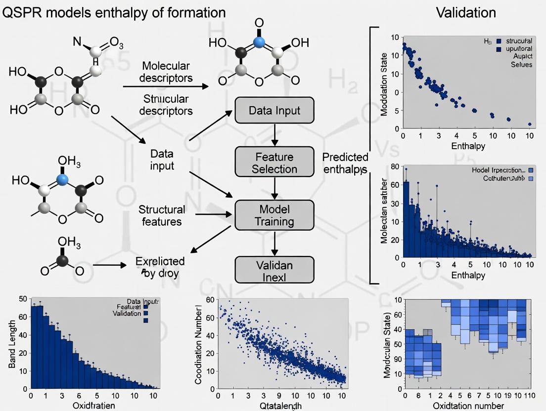
Workflow Visualization
QSPR Modeling Workflow: The established protocol for developing predictive models for ΔHf° encompasses data curation, computational preparation, descriptor processing, and model building with rigorous validation.
The standard enthalpy of formation represents a cornerstone property in energetic materials design, with QSPR methodologies providing powerful predictive tools for accelerating discovery and optimization. The integration of traditional QSPR with machine learning algorithms and first-principles computational methods has created a robust framework for ΔHf° prediction across diverse chemical spaces, including challenging inorganic and organometallic systems. As these computational approaches continue to evolve, their integration into automated screening workflows will further transform the paradigm of energetic materials development, enabling more efficient identification of high-performance, low-sensitivity compounds for advanced applications.
Key Differences Between Organic and Inorganic QSPR Modeling Approaches
Quantitative Structure-Property Relationship (QSPR) modeling serves as a fundamental computational tool for predicting the physicochemical properties of chemical compounds. While extensively developed for organic molecules, the application of QSPR to inorganic compounds presents unique challenges and methodological considerations. This application note delineates the key differences between organic and inorganic QSPR modeling approaches, with particular emphasis on predicting the standard enthalpy of formation (ΔHf°). Understanding these distinctions is crucial for researchers developing accurate predictive models for inorganic and organometallic systems, which are increasingly relevant in materials science, catalysis, and medicinal chemistry.
Fundamental Divergences in Modeling Approaches
Data Availability and Compositional Complexity
The most fundamental difference lies in the availability and nature of chemical data. Organic QSPR benefits from extensive, well-curated databases containing numerous structurally diverse carbon-based compounds, enabling robust model development [7]. In contrast, inorganic QSPR faces significantly more modest databases in both quantity and compositional variety [7]. This data scarcity is compounded by greater structural diversity in bonding patterns, coordination environments, and the inclusion of metallic elements, presenting substantial challenges for comprehensive descriptor representation.
Representation of Molecular Structure
Organic compounds are typically represented using simplified molecular input line entry system (SMILES) notations or topological descriptors that effectively capture covalent bonding patterns [7] [10]. For inorganic compounds, especially organometallic complexes and coordination compounds, structural representation must accommodate coordination bonds, varied oxidation states, and often requires specialized descriptor systems capable of handling stereochemical complexity [10]. The Simplex Representation of Molecular Structure (SiRMS) has emerged as a valuable approach for describing inorganic and chiral molecules by representing them as systems of simplexes (molecular multiplex), enabling comprehensive stereochemical analysis [10].
Table 1: Comparative Analysis of QSPR Approaches for Organic vs. Inorganic Compounds
| Characteristic | Organic QSPR | Inorganic QSPR |
|---|---|---|
| Data Availability | Extensive databases | Limited, modest databases |
| Structural Representation | SMILES, topological descriptors | SMILES with extensions, SiRMS, specialized descriptors |
| Descriptor Optimization | Standard correlation weights | Requires advanced optimization (CCCP, IIC) |
| Salts Handling | Often disregarded or transformed to neutral form | Must accommodate ionic character, often as disconnected structures |
| Common Software | Multiple well-established options | CORAL software adaptation, specialized tools |
| Model Validation | Standard train-test splits | Often requires specialized splits (active/passive training, calibration) |
Protocol for Inorganic Compound Enthalpy of Formation Modeling
Dataset Preparation and Curated Splitting
For modeling inorganic compound enthalpy of formation, implement the following protocol:
Data Curation: Collect standard enthalpy of formation (ΔHf°) values from reliable sources such as the DIPPR 801 database, which contains validated thermodynamic properties [6]. For organometallic complexes, ensure consistent experimental conditions and measurement methodologies.
Structured Data Splitting: Utilize the Las Vegas algorithm to partition data into four distinct subsets [7]:
- Active Training Set: Used for primary optimization of correlation weights
- Passive Training Set: Evaluates suitability of correlation weights for unseen compounds
- Calibration Set: Identifies optimization stagnation points
- Validation Set: Provides final model evaluation on completely unseen data
Split Proportions: For enthalpy of formation modeling, employ splits of 35% (active training), 35% (passive training), 15% (calibration), and 15% (validation) [7].
Descriptor Calculation and Optimization
Descriptor Selection: Employ Correlation Weight Descriptors (DCW) with parameters (3,15) for optimal representation of inorganic compounds [7]. For organometallic enthalpy of formation, key descriptors may include:
- Number of non-hydrogen atoms (nSK)
- Sum of conventional bond orders (SCBO)
- Number of oxygen atoms (nO)
- Number of fluorine atoms (nF)
- Number of heavy atoms (nHM) [6]
Optimization Target Functions: Implement two alternative optimization approaches:
- TF1: Optimization using Index of Ideality of Correlation (IIC)
- TF2: Optimization using Coefficient of Conformism of Correlative Prediction (CCCP)
Monte Carlo Optimization: Apply the Monte Carlo method for correlation weight optimization, with preference for CCCP (TF2) for enthalpy of formation models based on superior predictive performance [7].
Advanced Methodological Considerations
Target Function Selection for Optimal Predictive Performance
Comparative studies reveal distinct performance advantages for different target functions depending on the endpoint being modeled:
For octanol-water partition coefficient of mixed organic/inorganic sets and enthalpy of formation of organometallic compounds, TF2 (CCCP optimization) demonstrates superior predictive potential [7].
For acute toxicity (pLD50) in rats, TF1 (IIC optimization) yields preferable results, as TF2 approaches produced validation coefficients near zero [7].
This endpoint-specific performance highlights the necessity of empirical target function evaluation during model development.
Handling Stereochemical Complexity in Inorganic Systems
Inorganic and organometallic compounds frequently exhibit complex stereochemistry that must be adequately captured in QSPR models:
Simplex Representation: Implement the SiRMS approach to represent chiral centers using 5 simplexes, with atoms assigned canonical numbers according to established algorithms [10].
Stereochemical Configuration: Apply modified Kahn-Ingold-Prelog rules to identify R, S, and achiral configurations within the simplex framework [10].
Topicity Assessment: Evaluate stereochemical relationships between molecular fragments by analyzing simplex sequences, particularly crucial for coordination compounds with multiple chiral elements [10].
Table 2: Research Reagent Solutions for QSPR Modeling
| Research Reagent | Function | Application Notes |
|---|---|---|
| CORAL Software | QSPR/QSAR model development | Specialized adaptation for inorganic compounds; implements Monte Carlo optimization with CCCP/IIC target functions [7] |
| Dragon Software | Molecular descriptor calculation | Computes 1664+ molecular descriptors; requires preprocessing to remove non-informative descriptors [6] |
| SiRMS Package | Stereochemical analysis and representation | Essential for handling chiral inorganic complexes; enables multiplex representation of molecular structure [10] |
| Hyperchem Software | Molecular structure optimization | Performs geometry optimization using MM+ and PM3 methods prior to descriptor calculation [6] |
| GA-MLR Algorithms | Genetic algorithm-based multivariate linear regression | Develops linear models with optimal descriptor selection; particularly effective for enthalpy prediction [6] |
Validation Framework for Inorganic QSPR Models
Establish rigorous validation protocols specifically adapted for inorganic compounds:
Internal Validation:
External Validation:
Applicability Domain Assessment:
Comparative Performance Metrics:
The QSPR modeling of inorganic compounds demands specialized approaches distinct from organic chemistry applications. Critical differentiators include handling limited databases, representing complex bonding environments, accommodating stereochemical complexity, and implementing specialized optimization target functions. For enthalpy of formation prediction specifically, the combination of structured data splitting using Las Vegas algorithms, DCW(3,15) descriptors, and CCCP optimization (TF2) provides a robust methodological framework. Successful implementation requires both adaptation of existing organic QSPR protocols and development of inorganic-specific solutions, particularly for handling coordination compounds, organometallic complexes, and their unique stereochemical features.
Quantitative Structure-Property Relationship (QSPR) modeling for inorganic compounds and organometallics presents a unique set of challenges that distinguish it from its organic chemistry counterpart. Researchers pursuing QSPR models for inorganic compound enthalpy of formation confront a "modeling trilemma" centered on three interconnected issues: significant database limitations, exceptional structural complexity, and the problematic representation of salts [7]. While organic chemistry benefits from numerous extensive databases containing millions of compounds with well-curated properties, inorganic QSPR modeling operates with "considerably modest" databases in both number and content [7]. This data scarcity problem is further compounded by the structural diversity of inorganic compounds, which often contain metals, complex stereochemistry, and varied bonding patterns that defy simple descriptor systems. Additionally, the representation of ionic compounds and salts remains particularly challenging, as standard molecular representation approaches often fail to adequately capture their discontinuous nature [7]. This application note examines these core challenges and provides detailed protocols to advance QSPR research for inorganic compound enthalpy of formation.
Database Limitations: The Data Scarcity Problem
The Inorganic Data Landscape
The development of robust QSPR models requires large, high-quality datasets, which are notably scarce for inorganic compounds compared to organic substances. The fundamental challenge stems from the fact that "databases related to inorganic compounds are considerably modest in both their general number and contents" [7]. This data scarcity creates a significant bottleneck for training and validating models with sufficient chemical diversity.
Table 1: Comparative Analysis of Database Challenges in QSPR Modeling
| Aspect | Organic Compounds | Inorganic Compounds |
|---|---|---|
| Database Availability | Multiple extensive databases available | Few specialized databases |
| Data Points | Often thousands to millions of compounds | Typically hundreds of compounds |
| Property Coverage | Broad spectrum of measured properties | Limited properties measured |
| Structural Diversity | High within defined frameworks | Extreme variation with metals |
| Standardization | Well-established representation systems | Multiple representation challenges |
The problem is particularly acute for enthalpy of formation data, where experimental determination is complex, costly, and requires stringent conditions [12]. This experimental burden directly limits the available data for model development. For example, in the case of mercury compounds, which speciate in the environment, "insufficient mercury-species specific data was obtained, to conduct QSAR modelling successfully" [13]. This highlights a significant lack of data for even environmentally significant heavy metals.
Protocol: Handling Sparse Data for Enthalpy Modeling
Experimental Protocol 1: Data Augmentation and Curation for Inorganic Enthalpy of Formation
Purpose: To systematically collect, curate, and augment scarce experimental data for developing QSPR models of inorganic compound enthalpy of formation.
Materials and Reagents:
- CORAL software QSPR platform
- RDKit or OpenBabel for descriptor calculation
- Python/R with scikit-learn for model development
- Experimental databases: NIST Chemistry WebBook, ICSD, Pauling File
Procedure:
- Data Collection and Curation:
- Identify relevant enthalpy of formation data from experimental databases and literature.
- Apply strict quality filters: exclude data with undefined experimental conditions or purity concerns.
- Resolve identifier inconsistencies (e.g., CAS numbers, chemical names) through structure verification.
Data Augmentation:
- Apply group contribution methods as a preliminary estimation technique for missing data points [12].
- Use quantum chemical methods (G4, CBS-QB3, DFT) to compute formation enthalpies for compounds lacking experimental data [12].
- Implement similarity-based imputation using k-nearest neighbors within chemical families.
Dataset Division:
- Utilize the Las Vegas algorithm or Kennard-Stone algorithm to split data into representative subsets [7] [14].
- Divide data into: active training set (for model building), passive training set (for correlation weight optimization), calibration set (to detect stagnation), and validation set (for final evaluation) [7].
- Maintain chemical diversity across splits by ensuring each subset contains representatives of all major compound classes.
Validation Framework:
- Implement repeated cross-validation with multiple random splits to assess model stability on small datasets.
- Use Y-randomization tests to confirm model significance not arising from chance correlations.
- Define applicability domains using descriptor ranges present in the training set.
Diagram 1: Data Handling Protocol for Sparse Inorganic Datasets
Structural Complexity: Beyond Organic Descriptors
The Descriptor Challenge for Inorganic Systems
The structural complexity of inorganic compounds presents fundamental challenges for traditional QSPR descriptor systems. While organic compounds predominantly feature carbon-based skeletons with hydrogen, oxygen, and nitrogen atoms, inorganic compounds incorporate diverse metals, varied coordination geometries, and complex stereochemical arrangements that standard descriptor systems often fail to capture adequately [7]. This descriptor gap significantly complicates the development of predictive models for properties like enthalpy of formation.
The Simplex Representation of Molecular Structure (SiRMS) approach offers a potential solution by representing molecules as systems of simplexes (molecular multiplex), which can better capture stereochemical complexity [10]. This method can represent any 3D structure and account for stereochemical peculiarities, making it particularly valuable for inorganic compounds with complex chirality and coordination environments [10]. For organometallic complexes and coordination compounds, this approach enables a more comprehensive description of the stereochemical configuration beyond traditional organic descriptors.
Table 2: Molecular Descriptor Systems for Inorganic QSPR
| Descriptor Type | Application to Inorganic Compounds | Limitations |
|---|---|---|
| Topological Indices (Wiener, Gutman, Estrada) | Predicts combustion enthalpy of organic compounds; applicable to organometallics [12] | Limited capture of metal-centered geometry |
| Simplex Descriptors (SiRMS) | Handles stereochemistry and chirality in complex molecules [10] | Computational intensity for large systems |
| Graph Theory-Based Descriptors | Models carbon allotropes and nanomaterials [15] | Limited translation to coordination compounds |
| Group Contribution Methods | Estimates formation enthalpy from functional groups [12] | Limited parameters for metal-containing groups |
Protocol: Advanced Descriptor Implementation
Experimental Protocol 2: Handling Structural Complexity for Enthalpy Prediction
Purpose: To implement descriptor systems capable of capturing the structural complexity of inorganic compounds for enthalpy of formation prediction.
Materials and Reagents:
- CORAL software with SMILES representation capability
- SiRMS platform for stereochemical descriptors
- RDKit for topological descriptor calculation
- Python with NumPy, pandas, and scikit-learn for descriptor analysis
Procedure:
- Multi-Representation Approach:
- Generate SMILES strings for all compounds, ensuring proper representation of coordination environments.
- Calculate traditional 2D descriptors (topological, electronic, geometric) using standard cheminformatics tools.
- Implement SiRMS descriptors to capture stereochemical features and chirality elements [10].
- Compute special-purpose descriptors for organometallic complexes, focusing on metal-ligand bonding patterns.
Descriptor Selection and Optimization:
- Apply Monte Carlo optimization of correlation weights for different descriptor types [7].
- Use target functions like the Index of Ideality of Correlation (IIC) or Coefficient of Conformism of Correlative Prediction (CCCP) to guide optimization [7].
- Perform feature selection using genetic algorithms or stepwise regression to identify most relevant descriptors for enthalpy prediction.
Model Building with Complex Descriptors:
- Develop separate models for different inorganic compound classes (e.g., coordination compounds, organometallics, extended solids).
- Ensemble multiple descriptor types to capture complementary structural information.
- Validate model performance across different structural motifs to ensure generalizability.
Diagram 2: Multi-Descriptor Approach for Structural Complexity
Salt Representation: The Ionic Compound Challenge
The Representation Problem for Ionic Species
Salt representation presents a fundamental challenge in inorganic QSPR modeling, particularly for enthalpy of formation studies. As noted in recent research, "salts are usually represented as a disconnected structure, with two separate parts, and this represents a complication for modeling in most cases" [7]. This disconnected nature of ionic compounds contradicts the fundamental assumption of connectivity in most molecular representation systems, creating significant obstacles for descriptor calculation and model development.
The problem extends to practical applications, as "the most common software used to predict the properties of substances deals with organic substances and cannot be used for salts" [7]. This software limitation necessitates specialized approaches for ionic compounds, including ionic liquids and coordination salts. Research on ionic liquids has advanced this field, with studies developing QSPR models for properties like melting point by calculating descriptors for individual ions and combining them using appropriate rules [16]. However, these approaches require careful consideration of how to appropriately combine cationic and anionic descriptors to represent the salt as a whole.
Protocol: Salt Representation and Modeling
Experimental Protocol 3: QSPR Modeling for Ionic Compounds and Salts
Purpose: To develop effective QSPR models for ionic compounds and salts, addressing their unique representation challenges for enthalpy of formation prediction.
Materials and Reagents:
- CORAL software or custom QSPR platform with salt handling capability
- Quantum chemistry software (Gaussian, ORCA) for partial charge calculation
- In-house scripts for descriptor combination rules
- Ionic liquid databases for method validation
Procedure:
- Salt Representation and Descriptor Calculation:
- Represent salts as disconnected structures with separate cationic and anionic components.
- Calculate descriptors separately for cations and anions using standard molecular representation.
- Implement combining rules to generate salt descriptors from individual ion descriptors:
- Arithmetic mean: ( D{salt} = \frac{D{cation} + D{anion}}{2} )
- Geometric mean: ( D{salt} = \sqrt{D{cation} \times D{anion}} )
- Sum: ( D{salt} = D{cation} + D_{anion} )
- Custom combination rules based on chemical intuition
Ion-Specific Descriptors:
- Calculate electrostatic potential-derived descriptors for each ion.
- Include size and shape descriptors for both cations and anions.
- Compute interaction potential descriptors capturing cation-anion complementarity.
Model Development and Validation:
- Develop models using different descriptor combination rules.
- Validate model performance on diverse salt systems including ionic liquids, coordination compounds, and simple salts.
- Compare performance across different chemical families to identify optimal approaches.
- Define applicability domains specifically for ionic compound space.
Integrated Workflow: A Path Forward
Comprehensive Modeling Strategy
Addressing the interconnected challenges of database limitations, structural complexity, and salt representation requires an integrated workflow that leverages recent methodological advances. The most promising approach combines careful data handling, advanced descriptor systems, and specialized representation methods tailored to inorganic compounds.
Table 3: Research Reagent Solutions for Inorganic QSPR
| Research Reagent | Function | Application in Inorganic QSPR |
|---|---|---|
| CORAL Software | QSPR model development with Monte Carlo optimization | Building models for organic and inorganic substances with optimized correlation weights [7] |
| SiRMS Platform | Stereochemical analysis and descriptor calculation | Handling chiral inorganic complexes and stereochemical complexity [10] |
| RDKit | Cheminformatics and descriptor calculation | Calculating standard molecular descriptors for organometallic compounds |
| Quantum Chemistry Codes (Gaussian, ORCA) | Electronic structure calculation | Generating quantum chemical descriptors and validating experimental data [12] |
| Topological Index Algorithms | Graph-theoretical descriptor calculation | Modeling carbon allotropes and nanomaterials [15] |
Unified Experimental Protocol
Integrated Protocol: Comprehensive QSPR for Inorganic Enthalpy of Formation
Purpose: To provide an integrated workflow addressing database, complexity, and representation challenges for predicting inorganic compound enthalpy of formation.
Procedure:
- Data Compilation and Curation:
- Implement Protocol 1 for data collection, augmentation, and division.
- Apply strict quality control measures and resolve representation inconsistencies.
- Use Las Vegas algorithm for creating balanced splits across compound classes.
Multi-Scale Descriptor Calculation:
- Implement Protocol 2 for comprehensive descriptor calculation.
- Combine traditional 2D descriptors, SiRMS stereochemical descriptors, and quantum chemical descriptors.
- For ionic compounds, implement Protocol 3 for salt representation and descriptor combination.
Model Development and Optimization:
- Optimize correlation weights using Monte Carlo method with target functions (IIC or CCCP) [7].
- Develop ensemble models combining different descriptor types and representation approaches.
- Validate models using rigorous cross-validation and external validation sets.
Model Interpretation and Application:
- Analyze descriptor contributions to identify key structural factors influencing enthalpy of formation.
- Define applicability domains for reliable prediction.
- Implement models for virtual screening and compound design.
Diagram 3: Integrated Workflow for Inorganic QSPR Modeling
The development of accurate QSPR models for inorganic compound enthalpy of formation requires addressing three fundamental challenges: limited database availability, exceptional structural complexity, and problematic salt representation. Through specialized protocols for data handling, advanced descriptor systems, and tailored representation approaches, researchers can overcome these limitations. The integrated workflow presented here provides a path forward for developing predictive models that account for the unique characteristics of inorganic compounds, ultimately enabling more efficient discovery and design of novel materials with tailored thermodynamic properties.
Comparative Analysis of QSPR vs. Traditional Group Contribution Methods for Inorganics
The accurate prediction of thermodynamic properties, such as the standard enthalpy of formation (ΔHf°), is fundamental to advancements in inorganic chemistry, materials science, and drug development. This property, defined as the enthalpy change when one mole of a compound is formed from its constituent elements in their standard states, serves as a critical parameter for assessing chemical reactivity and stability [6]. For researchers working with inorganic compounds, the experimental determination of ΔHf° is often labor-intensive, costly, and sometimes hazardous, creating a significant need for reliable predictive computational methods [17].
Within this context, two primary computational approaches have emerged: traditional Group Contribution Methods (GCMs) and Quantitative Structure-Property Relationship (QSPR) models. This application note provides a detailed comparative analysis of these methodologies, focusing on their underlying principles, accuracy, and practical application for predicting the enthalpy of formation of inorganic and organometallic compounds. The analysis is situated within a broader thesis on the development of robust QSPR models for inorganic compounds, aiming to equip researchers with the knowledge to select and implement the most appropriate predictive strategy for their work.
Traditional Group Contribution Methods (GCMs)
Core Principle: GCMs operate on an additive principle, where a molecule is decomposed into fundamental structural subunits (functional groups or atoms). The target property is estimated by summing the predetermined contributions of these subunits [18] [19].
Mechanism: The property ( P ) is calculated using the general formula:
( P = \sum{i} n{i} C_{i} )
where ( n{i} ) is the number of occurrences of group ( i ), and ( C{i} ) is its contribution value [18]. For more complex models, particularly for mixture properties, group-interaction parameters (( G{ij} )) are introduced, where ( P = f(G{ij}) ) [18].
Key Characteristics:
- Descriptors Used: Pre-defined functional groups or atoms (e.g., -OH, =O, carbon atoms, metal centers) [20].
- Training Data: Relies on experimental property data to regress the contribution values (( C_{i} )) for each group [18].
- Applicability: Limited to compounds consisting only of groups for which contribution parameters have been previously determined. This is a significant bottleneck for novel inorganic complexes [7] [19].
Quantitative Structure-Property Relationship (QSPR) Models
Core Principle: QSPR models establish a mathematical correlation between a diverse set of numerical descriptors, derived directly from the molecular structure, and the target property [7] [6].
Mechanism: A statistical or machine-learning model is trained to map structural descriptors to the property value.
( P = F(D1, D2, ..., D_m) )
where ( F ) is the model function and ( D1 ) to ( Dm ) are the molecular descriptors [6].
Key Characteristics:
- Descriptors Used: Can be topological indices, quantum chemical descriptors (e.g., molecular polarizability, atomic charges), or "norm indices" calculated from atomic property matrices [21] [22] [23]. These descriptors often have defined physical meanings [23].
- Training Data: Uses experimental data to learn the function ( F ) that best relates the descriptors to the property.
- Applicability: Highly generalizable. Models can predict properties for any structure, including novel molecules, as long as the required descriptors can be calculated [7] [6].
Workflow Comparison
The following diagram illustrates the fundamental procedural differences between GCM and QSPR methodologies.
Quantitative Performance Comparison
A critical evaluation of predictive accuracy reveals distinct performance differences between GCMs and QSPR models, particularly for complex or novel compounds.
Table 1: Comparison of Predictive Accuracy for Enthalpy-related Properties
| Prediction Method | Substances | Key Parameter | RMSE | R² | Reference |
|---|---|---|---|---|---|
| Traditional GCM | Nitro Compounds | ΔH (J/g) | 2280 | 0.09 | [17] |
| Traditional GCM | Organic Peroxides | ΔH (J/g) | 2030 | 0.08 | [17] |
| QSPR Model | Organic Peroxides | ΔH (J/g) | 113 | 0.90 | [17] |
| QSPR Model | Self-reactive Substances | ΔH (kJ/mol) | 52 | 0.85 | [17] |
| QSPR (GA-MLR) | 1115 Diverse Compounds | ΔHf° (kJ/mol) | ~58.5* | 0.983 | [6] |
Note: RMSE estimated from standard deviation (s) reported in the source.
The data demonstrates that QSPR models achieve significantly higher accuracy and lower error compared to traditional GCMs. The QSPR model developed for 1115 compounds using a genetic algorithm-based multivariate linear regression (GA-MLR) is particularly noteworthy for its high coefficient of determination (R² = 0.983), indicating an excellent fit and strong predictive capability [6].
Detailed Experimental Protocols
Protocol 1: Implementing a QSPR Model for ΔHf° Prediction
This protocol outlines the steps to develop a QSPR model for standard enthalpy of formation, based on the method described by [6].
Data Compilation
- Source a large, high-quality dataset of experimental ΔHf° values. The DIPPR 801 database, recommended by AIChE, is a standard source [6].
- Select a diverse set of compounds (e.g., 1000+), ensuring coverage of various chemical families to enhance model generalizability.
Molecular Structure Optimization and Descriptor Calculation
- Draw and pre-optimize the 2D/3D chemical structures of all compounds using software like Hyperchem.
- Perform a more precise geometry optimization using a semi-empirical method (e.g., PM3) or density functional theory (DFT).
- Use specialized software (e.g., Dragon) to calculate a comprehensive set of molecular descriptors (1600+). This yields descriptors encoding topological, geometric, and electronic information.
Descriptor Selection and Model Building
- Pre-process the descriptor matrix: remove descriptors with near-constant values, those that are highly correlated, or those with missing values.
- Split the dataset randomly into a training set (e.g., 80%) for model development and a test set (e.g., 20%) for final validation.
- Apply a variable selection algorithm like Genetic Algorithm-Multivariate Linear Regression (GA-MLR) to the training set to identify the optimal subset of descriptors that best predict ΔHf°.
Model Validation
- Internal Validation: Use cross-validation (e.g., Leave-One-Out) on the training set to calculate Q² and assess robustness.
- External Validation: Apply the final model to the untouched test set and calculate statistical metrics (R², RMSE) to evaluate its true predictive power [6].
Protocol 2: Applying a Group Contribution Method
This protocol describes the standard procedure for using an existing GCM to estimate ΔHf°.
Molecular Decomposition
Parameter Retrieval
- From the GCM's published tables, retrieve the contribution value (( C_i )) for each identified group.
Property Calculation
- Insert the group counts (( ni )) and contribution values (( Ci )) into the model's equation.
- Sum the contributions to obtain the estimated ΔHf°.
Limitation Note: This method will fail if the target compound contains functional groups not parameterized in the chosen GCM, a common issue with novel inorganic compounds [7].
The Scientist's Toolkit: Essential Research Reagents & Software
Table 2: Key Resources for Enthalpy Prediction Studies
| Category / Item | Specific Examples | Function / Application |
|---|---|---|
| Experimental Data Sources | DIPPR 801 Database, NIST Chemistry WebBook, CRC Handbook | Provide high-quality, critically evaluated experimental thermochemical data for model training and validation. |
| Structure Optimization & QC Calculation | Hyperchem, Gaussian 09 (GEDIIS/GDIIS optimizer) | Used for drawing molecular structures and performing quantum chemical calculations to obtain optimized geometries and quantum chemical descriptors [6] [23]. |
| Molecular Descriptor Generators | Dragon Software, AlvaDesc, RDKit | Calculate thousands of molecular descriptors (topological, constitutional, quantum-chemical) from molecular structure for QSPR model development [6] [22]. |
| QSPR Modeling Software | CORAL Software, MATLAB | Provide environments for building QSPR models, utilizing algorithms like Monte Carlo optimization or Genetic Algorithm (GA-MLR) for descriptor selection and model training [7] [6]. |
| Group Contribution Methods | Joback Method, Ambrose Method, Marrero-Gani Method | Established GCMs containing parameter tables for estimating various pure-component properties, including critical constants and enthalpies of formation [18] [19] [6]. |
The comparative analysis presented in this application note demonstrates a clear paradigm shift in the prediction of enthalpic properties for inorganic compounds. Traditional Group Contribution Methods, while simple and easy to implement, are constrained by their dependence on pre-defined groups, leading to limited applicability and lower predictive accuracy for chemistries extending beyond their parameterization set [17] [7].
In contrast, modern QSPR approaches, leveraging data-driven algorithms and sophisticated molecular descriptors, offer superior accuracy, robustness, and generalizability. The integration of machine learning techniques, such as genetic algorithms and random forests, is poised to further overcome existing challenges like limited sample sizes [17] [23]. For researchers engaged in the development of new inorganic compounds or materials, QSPR models represent the more powerful and future-proof toolkit, enabling reliable in silico property estimation that can significantly accelerate the design and discovery process.
Essential Molecular Descriptors for Characterizing Inorganic and Organometallic Systems
The development of robust Quantitative Structure-Property Relationship (QSPR) models for inorganic and organometallic compounds presents unique challenges compared to organic molecular systems. While organic QSPR/QSAR studies benefit from extensive databases and well-established descriptor sets, inorganic compounds have historically received less attention, with many conventional software tools limited to organic structures [7]. The fundamental distinction lies in molecular architecture: inorganic compounds typically feature smaller structures containing metals, oxygen, nitrogen, sulfur, and phosphorus, rather than the complex carbon chains dominant in organic chemistry [7]. This application note delineates essential molecular descriptors and protocols specifically validated for inorganic and organometallic systems, with particular emphasis on enthalpy of formation prediction within broader QSPR research frameworks.
Essential Molecular Descriptors for Inorganic Systems
The descriptor selection process must accommodate the distinctive structural features of inorganic compounds, including metal centers, coordination geometries, and ligand environments. Based on recent research, the following descriptor categories have demonstrated significant predictive value for inorganic and organometallic systems.
Table 1: Essential Molecular Descriptors for Inorganic and Organometallic QSPR Models
| Descriptor Category | Specific Examples | Application in Inorganic Systems | Relationship to Enthalpy of Formation |
|---|---|---|---|
| Composition-Based | Number of non-hydrogen atoms (nSK), Number of specific heteroatoms (nO, nF), Number of heavy atoms (nHM) [6] | Fundamental for characterizing elemental composition and stoichiometry in inorganic complexes and organometallics | Direct correlation with molecular complexity and bond energy contributions [6] |
| Topological & Connectivity | Sum of conventional bond orders (SCBO) [6], Molecular fingerprints (Morgan, Atompairs) [24] | Encodes bond characteristics and connectivity patterns around metal centers | Reflects overall bonding environment and stability [6] |
| Geometric & Surface-Based | Molecular surface area, Molecular volume (V), Polar surface area (PSA), Topological polar surface area (TPSA) [25] | Captures spatial requirements and surface properties influenced by metal coordination | Correlates with intermolecular interaction energies in crystalline phases [25] |
| Electronic & Electrostatic | Fractional charged partial surface area (FPSA3) [25], Electrostatic variance parameters (σ²₋, σ²₊) [25] | Characterizes charge distribution and electrostatic potential around metal complexes | Indicates ionic character and metal-ligand bond strength [25] |
| Specialized Inorganic | Metal type and oxidation state, Coordination number, Ligand field parameters | Specifically designed for transition metal complexes and coordination compounds | Directly impacts stability and bond energetics in coordination spheres |
For researchers requiring interpretable models, specialized substructure sets like Saagar offer chemically viable functional groups and moieties systematically gathered from literature, demonstrating particular utility in building transparent QSAR/QSPR models [26].
Experimental Protocols for QSPR Model Development
Protocol 1: QSPR Model Construction Using CORAL Software
This protocol outlines the methodology for developing QSPR models for inorganic compounds using the CORAL software, as validated for endpoints including octanol-water partition coefficient and enthalpy of formation [7].
Workflow Overview:
Step-by-Step Procedure:
Data Set Preparation
- Compile experimental values for the target property (e.g., standard enthalpy of formation, ΔHf°) from validated databases such as DIPPR 801 [6].
- Represent molecular structures using Simplified Molecular Input Line Entry System (SMILES) notation. For inorganic compounds and metal complexes, ensure accurate representation of metal atoms and coordination environments.
Descriptor Calculation
- Calculate optimal descriptors using the Correlation Weights (DCW) approach within CORAL software. The DCW(n,m) parameters define the scope of the SMILES attributes accounted for, where 'n' represents the number of epochs of optimization and 'm' defines the number of symbols in the SMILES [7].
- Common settings include DCW(3,15) for diverse datasets and DCW(1,15) for specific endpoints like toxicity [7].
Stochastic Data Splitting
- Partition the data set into four distinct subsets using the Las Vegas algorithm [7]:
- Active Training Set: Used for correlation weight optimization.
- Passive Training Set: Validates suitability of correlation weights for compounds not involved in optimization.
- Calibration Set: Monitors for stagnation during optimization.
- Validation Set: Provides final evaluation of model predictive potential.
- Implement multiple random splits (typically 3-4) to ensure model robustness and avoid split-specific artifacts.
- Partition the data set into four distinct subsets using the Las Vegas algorithm [7]:
Correlation Weight Optimization
- Optimize correlation weights using the Monte Carlo method with one of two target functions [7]:
- TF1: Maximizes the Index of Ideality of Correlation (IIC)
- TF2: Maximizes the Coefficient of Conformism of a Correlative Prediction (CCCP)
- Selection criteria: TF2 (CCCP) generally provides superior predictive potential for physicochemical properties like octanol-water partition coefficient and enthalpy of formation, while TF1 (IIC) may be preferred for toxicity endpoints [7].
- Optimize correlation weights using the Monte Carlo method with one of two target functions [7]:
Model Validation
- Evaluate model performance using standard statistical measures: coefficient of determination (R²), root mean square error (RMSE), and cross-validated correlation coefficient (Q²) [7] [6].
- Apply Y-randomization testing to confirm model significance and external validation with completely excluded compounds to verify predictive power [6].
Protocol 2: GA-MLR Modeling for Enthalpy of Formation Prediction
This protocol details an alternative approach using Genetic Algorithm-based Multivariate Linear Regression (GA-MLR), successfully applied to predict standard enthalpy of formation for 1,115 diverse compounds [6].
Workflow Overview:
Step-by-Step Procedure:
Molecular Structure Optimization
- Draw chemical structures using molecular modeling software (e.g., Hyperchem).
- Perform preliminary geometry optimization using molecular mechanics force fields (e.g., MM+).
- Execute more precise optimization using semi-empirical methods (e.g., PM3) or density functional theory (e.g., B3LYP/6-31G(d)) [6] [25].
Descriptor Calculation and Filtering
- Calculate molecular descriptors using comprehensive software packages (e.g., Dragon, which can compute 1,664 molecular descriptors) [6].
- Apply descriptor filtering to eliminate non-informative variables:
- Remove descriptors with standard deviation < 0.0001 (near-constant values).
- Eliminate descriptors with only one value different from remaining ones.
- Exclude one descriptor from each highly correlated pair (correlation coefficient ≥ 0.95).
Genetic Algorithm Descriptor Selection
- Implement genetic algorithm for variable selection to identify the most relevant descriptor subset.
- Use cross-validated correlation coefficient (Q²) as the fitness function to guide descriptor selection.
- Iteratively increase model complexity until additional descriptors no longer significantly improve Q².
Multivariate Linear Regression Model Building
- Construct the final QSPR model using the form: ΔHf° = Intercept + Σ(bᵢ × Descriptorᵢ)
- For the published 1,115 compound model, the equation was [6]: ΔHf° = 50.1688 - 80.52012 × nSK + 53.64546 × SCBO - 169.21889 × nO - 174.75477 × nF - 266.57659 × nHM
Comprehensive Model Validation
- Apply leave-one-out cross-validation to calculate Q².
- Perform external validation with a pre-selected test set (typically 20% of data) to determine external predictive ability (Q²ext).
- Conduct bootstrap validation (e.g., 5,000 repetitions) to assess model stability [6].
Performance Metrics and Validation
Table 2: Representative Performance Metrics for Inorganic Compound QSPR Models
| Model Endpoint | Compounds | Algorithm | Key Descriptors | R² | Q² | Reference |
|---|---|---|---|---|---|---|
| ΔHf° (Organic & Inorganic) | 1,115 | GA-MLR | nSK, SCBO, nO, nF, nHM | 0.983 | 0.983 | [6] |
| Octanol-Water (Inorganic Set) | 461 | CORAL (TF2) | DCW(3,15) | 0.85 | 0.82 | [7] |
| ΔHf° (Organometallic) | 122 | CORAL (TF2) | DCW(3,15) | 0.79 | 0.75 | [7] |
| Sublimation Enthalpy | 260 | MLR | SA, PSA, nROH | 0.97 | 0.96 | [25] |
| Drug Release (MOFs) | 67 | BMLR | nN, nO, IM-L | 0.999 | 0.999 | [27] |
Table 3: Essential Resources for Inorganic QSPR Modeling
| Resource Category | Specific Tools/Software | Primary Application | Key Features for Inorganic Chemistry |
|---|---|---|---|
| QSPR Modeling Software | CORAL software [7] | General QSPR model development | Implements Monte Carlo optimization; handles both organic and inorganic SMILES representations |
| Descriptor Calculation | Dragon software [6] | Molecular descriptor calculation | Calculates 1,664 molecular descriptors; requires pre-optimized structures |
| Descriptor Calculation | BioPPSy package [25] | QSPR model development | Includes descriptors for hydrophilicity (Hy), molecular volume (V), Zagreb index (ZM1) |
| Structure Optimization | Gaussian 09 [25] | Quantum chemical calculations | Geometry optimization at DFT levels (e.g., B3LYP/6-31G(d)); calculation of electronic descriptors |
| Structure Optimization | Hyperchem [6] | Molecular modeling | Structure drawing and preliminary optimization with MM+ and PM3 methods |
| Specialized Substructure Libraries | Saagar feature set [26] | Read-across and interpretable QSPR | 834 chemistry-aware substructures; includes organometallic motifs |
| Experimental Databases | DIPPR 801 [6] | Thermochemical data | Recommended source for standard enthalpy of formation values |
| Machine Learning Algorithms | XGBoost, RPropMLP [24] | Advanced QSPR modeling | Superior performance with traditional 1D-3D descriptors for ADME-Tox targets |
Advanced Modeling Techniques and Practical Implementation Strategies
The accurate prediction of the standard enthalpy of formation (ΔHf°) is a cornerstone in the development of new materials and compounds, particularly within the realm of inorganic and organometallic chemistry. This thermodynamic property, defined as the enthalpy change when one mole of a compound is formed from its constituent elements in their standard states, is crucial for assessing stability, reactivity, and energetic performance [6]. Traditional experimental determination of ΔHf° is often constrained by high costs, safety risks, and lengthy procedures, creating a significant bottleneck in research and development cycles [3]. Consequently, robust computational methods for predicting this property are of immense value.
Quantitative Structure-Property Relationship (QSPR) modeling has emerged as a powerful in silico alternative, establishing quantitative mappings between molecular structures and macroscopic properties [3]. The integration of machine learning (ML) has dramatically enhanced the predictive power of QSPR models. Unlike traditional linear regression, ML algorithms can decipher complex, non-linear relationships between molecular descriptors and target properties [28]. Among these, Random Forests and other ensemble methods have demonstrated superior performance for QSPR tasks, offering high accuracy, robustness against overfitting, and the ability to handle high-dimensional descriptor spaces [29] [30]. This protocol details the application of these ensemble methods specifically for predicting the enthalpy of formation of inorganic compounds, providing a structured framework for researchers to implement these powerful tools.
Application Notes & Experimental Protocols
Protocol: Random Forest Model for Enthalpy of Formation Prediction
This protocol provides a step-by-step methodology for developing a predictive QSPR model for the standard enthalpy of formation of inorganic and organometallic compounds using the Random Forest algorithm.
- Objective: To construct and validate a robust Random Forest regression model for predicting ΔHf°.
- Primary Application: Accelerated screening and stability evaluation of novel inorganic compounds in materials science and drug development [30].
Procedure:
Data Curation and Pre-processing
- Data Source: Compile a dataset of known ΔHf° values for inorganic/organometallic compounds from reliable databases such as DIPPR 801 or other thermochemical compilations [6]. For inorganic complexes, including Pt(IV) complexes, specialized datasets may be required [7].
- Data Splitting: Randomly split the dataset into three subsets:
- Alternative Splits: Some advanced approaches use a four-way split (e.g., active training, passive training, calibration, and validation sets) using algorithms like the Las Vegas algorithm for enhanced model validation [7].
Molecular Descriptor Calculation and Selection
- Structure Representation: Represent molecular structures using Simplified Molecular Input Line Entry System (SMILES) notations or generate optimized 2D/3D structures using software like Hyperchem [6].
- Descriptor Calculation: Use cheminformatics software such as Dragon, RDKit, or CORAL to calculate molecular descriptors [6] [7] [30]. These can include:
- Topological Descriptors: Wiener index, Gutman index, Estrada index, Zagreb indices, and Kappa shape indices [12] [30].
- Constitutional Descriptors: Number of non-hydrogen atoms (
nSK), number of specific heavy atoms (e.g.,nO,nF), number of rotatable bonds (NumRotatableBonds) [6] [30]. - Electronic Descriptors: Sum of conventional bond orders (
SCBO), valence connectivity indices (Chi1v) [6] [30].
- Feature Selection: To avoid overfitting and reduce computational cost, perform feature selection.
- Random Forest Importance: Use the built-in variable importance measure of Random Forest to rank descriptors. Retain the top-ranked descriptors that contribute most to predictive accuracy [29].
- Correlation Filtering: Remove descriptors with near-zero variance or those that are highly correlated (e.g., correlation coefficient > 0.95) with others [6].
Model Training and Validation
- Algorithm Implementation: Implement the Random Forest regressor using a scientific computing environment like Python with the Scikit-learn library.
- Hyperparameter Tuning: Optimize key hyperparameters using the validation set, for instance via grid search or random search. Critical parameters include:
n_estimators: Number of trees in the forest.max_depth: Maximum depth of each tree.min_samples_split: Minimum number of samples required to split a node.
- Model Validation: Employ rigorous validation techniques:
- k-Fold Cross-Validation: Assess model stability on the training set (e.g., 10-fold cross-validation) [29].
- External Validation: Use the held-out test set for the final performance report.
- Statistical Metrics: Calculate key performance indicators: R² (coefficient of determination), RMSE (Root Mean Square Error), MAE (Mean Absolute Error), and MAPE (Mean Absolute Percentage Error) [12] [29].
Logical Workflow:
The following diagram illustrates the sequential workflow for developing the Random Forest QSPR model.
Performance Data and Comparison
The table below summarizes the performance of various machine learning models, including ensemble methods, as reported in the literature for predicting enthalpies of formation and related properties.
Table 1: Performance Comparison of ML Models in QSPR Studies for Enthalpy Prediction
| Model | Dataset | Key Descriptors | Performance (Test Set) | Reference |
|---|---|---|---|---|
| Random Forest | 3477 Organic Compounds (Combustion Enthalpy) | Estrada Index, Gutman Index, Wiener Index | R² = 0.9810, RMSE = 551.9 kJ·mol⁻¹ | [12] |
| Gradient Boosting | Organic Semiconductors (Enthalpy of Formation) | Kappa2, NumRotatableBonds, frunbrchalkane | R² = 0.70 | [30] |
| Extra Trees | Organic Semiconductors (Enthalpy of Formation) | Kappa2, NumRotatableBonds, frunbrchalkane | R² = 0.68 | [30] |
| GA-MLR | 1115 Diverse Compounds (Enthalpy of Formation) | nSK, SCBO, nO, nF, nHM | R² = 0.9830, Q² = 0.9826 | [6] |
| Random Forest with Feature Selection | Hydrocarbons (Enthalpy of Formation) | 89 selected from 1485 descriptors | Improved RMSE (23% lower than no selection) | [29] |
Advanced Integration: Feature Selection with Random Forest
A critical challenge in QSPR is the "curse of dimensionality," where the number of molecular descriptors far exceeds the number of compounds. An advanced application of Random Forest is its use for feature selection prior to model building, which significantly enhances model interpretability and performance [29].
- Objective: To identify the most relevant molecular descriptors for predicting ΔHf°.
- Procedure:
- Preliminary Ranking: Calculate the importance of all descriptors using the standard Random Forest variable importance score (e.g., mean decrease in impurity).
- Elimination: Remove descriptors with negligible importance scores.
- Iterative Selection: Construct an ascending sequence of models by adding the top-ranked variables one by one. A variable is retained only if the error gain (e.g., decrease in OOB error or RMSE) exceeds a predefined threshold [29].
- Final Model Training: Train the final predictive model (e.g., Support Vector Machine or a new Random Forest) using the optimized, minimal descriptor subset.
Logical Workflow:
The feature selection process is outlined in the diagram below.
The Scientist's Toolkit: Research Reagent Solutions
Table 2: Essential Software and Computational Tools for ML-Driven QSPR
| Tool / Resource | Type | Primary Function in Protocol |
|---|---|---|
| Dragon | Software | Calculates a vast array (>1600) of molecular descriptors from molecular structure [6]. |
| RDKit | Cheminformatics Library | Open-source toolkit for cheminformatics, including descriptor calculation, fingerprint generation, and SMILES processing [30]. |
| CORAL Software | Software | Builds QSPR/QSAR models using SMILES and graph-based descriptors, with optimization via Monte Carlo methods [7]. |
| Scikit-learn (Python) | ML Library | Provides implementations of Random Forest, Gradient Boosting, and other ML algorithms, along with model validation tools [30]. |
| Hyperchem | Software | Used for molecular modeling, structure optimization, and preliminary geometry calculations [6]. |
Topological Descriptors and Graph Theory Applications for Inorganic Compounds
The application of topological descriptors and graph theory provides a powerful mathematical framework for modeling the physicochemical properties of inorganic and organometallic compounds within Quantitative Structure-Property Relationship (QSPR) studies. While traditionally more prevalent in organic chemistry, these computational approaches are increasingly demonstrating significant utility for inorganic systems, including the prediction of key thermodynamic properties such as the enthalpy of formation [7]. Chemical graph theory represents molecular structures as mathematical graphs, where atoms correspond to vertices and chemical bonds to edges, enabling the calculation of numerical topological indices that encode essential structural information [21] [12]. These descriptors serve as critical inputs for constructing robust QSPR models that can predict inorganic compound behavior with accuracy comparable to traditional quantum chemical methods, while offering substantial advantages in computational efficiency [7] [31]. This Application Note details established protocols for implementing these methodologies specifically for inorganic compounds, with particular emphasis on enthalpy of formation prediction within broader QSPR research initiatives.
Current Applications in Inorganic QSPR Modeling
Research demonstrates several successful applications of topological descriptors for predicting the properties of inorganic and organometallic compounds, effectively addressing the historical bias toward organic chemistry in QSPR studies [7].
Table 1: Application of Topological Descriptors in Inorganic Compound QSPR
| Compound Class | Predicted Property | Topological Descriptors Used | Model Performance |
|---|---|---|---|
| Organometallic Complexes [7] | Enthalpy of Formation | Correlation weights of SMILES attributes | Optimized via Monte Carlo method; CCCP optimization provided superior predictive potential |
| Platinum(IV) Complexes [7] | Octanol-Water Partition Coefficient (Log P) | DCW(3,15) descriptors from SMILES | Models built using active training, passive training, and calibration sets |
| Energetic Compounds [31] | Sublimation Enthalpy (ΔsubH) | Molecular Area (A), TPSA, nRNO₂, S | Topological descriptor-based models showed higher accuracy than quantum chemical descriptors |
| General Inorganic & Small Molecules [7] | Octanol-Water Partition Coefficient | Descriptors for Au, Ge, Hg, Pb, Se, Si, Sn-containing compounds | QSPR models developed for set containing specially defined inorganic substances |
Key advancements include the development of specialized descriptor optimization techniques such as the Index of Ideality of Correlation (IIC) and the Coefficient of Conformism of a Correlative Prediction (CCCP), which have improved model robustness for inorganic datasets [7]. Furthermore, the integration of topological descriptors with machine learning algorithms including XGBoost and Particle Swarm Optimization (PSO) has enabled accurate prediction of sublimation enthalpy for energetic inorganic compounds with minimal computational time investment [31].
Experimental Protocols and Methodologies
Protocol 1: QSPR Model Development for Inorganic Compound Enthalpy
This protocol outlines the workflow for developing a QSPR model to predict the enthalpy of formation for organometallic complexes using topological descriptors derived from SMILES notation [7].
Materials and Data Requirements:
- Dataset of Inorganic Compounds: Curated set of organometallic complexes with experimentally determined standard enthalpy of formation values (e.g., kJ/mol at 298.15 K and 1 bar).
- SMILES Representations: Simplified Molecular Input Line Entry System (SMILES) strings for all compounds in the dataset.
- Computational Software: CORAL software or equivalent QSPR modeling environment capable of calculating descriptors and optimizing correlation weights.
Procedure:
- Data Preparation and Splitting
- Compile a dataset of inorganic compounds with known experimental property values.
- Divide the dataset into four distinct subsets using a stochastic algorithm (e.g., Las Vegas algorithm):
- Active Training Set (∼35%): Used for primary optimization of correlation weights.
- Passive Training Set (∼35%): Used to validate the generalizability of correlation weights.
- Calibration Set (∼15%): Used to detect optimization stagnation.
- Validation Set (∼15%): Used for final, independent assessment of model predictive potential.
Descriptor Calculation and Optimization
- Calculate Descriptor of Correlation Weights (DCW) from the SMILES representations of compounds in the active training set. The DCW(3,15) configuration is typically employed.
- Optimize correlation weights using the Monte Carlo method with target function TF2, which utilizes the Coefficient of Conformism of a Correlative Prediction (CCCP), as it has been shown to provide superior predictive potential for inorganic compound enthalpy models [7].
Model Validation and Deployment
- Validate the optimized model against the passive training, calibration, and external validation sets.
- Assess model quality using statistical metrics: coefficient of determination (R²), mean absolute error (MAE), and root mean square error (RMSE).
- Deploy the validated model to predict enthalpy of formation for new, unknown inorganic compounds.
Protocol 2: Machine Learning-QSPR for Sublimation Enthalpy
This protocol describes the use of topological molecular descriptors with machine learning to predict the sublimation enthalpy of energetic inorganic compounds, a critical property for determining solid-phase enthalpy of formation [31].
Materials and Data Requirements:
- Extended Energetic Compounds Dataset: Augment standard databases (e.g., DIPPR 801) with experimental sublimation enthalpy data for nitro compounds and other energetic inorganic molecules.
- Topological Descriptors: Four key descriptors - Molecular Area (A), Topological Polar Surface Area (TPSA), Number of Nitro Groups (nRNO₂), and Molecular S-index (S).
- Machine Learning Environment: Python with libraries including XGBoost, Scikit-learn, and PSOFit.
Procedure:
- Dataset Construction and Preprocessing
- Compile a foundational dataset from standard databases, excluding metal-containing and non-neutral molecules.
- Supplement this dataset with experimentally measured sublimation enthalpies of energetic inorganic compounds from literature sources.
- Preprocess data to handle missing values and normalize descriptor ranges if necessary.
Descriptor Calculation and Selection
- Calculate the four topological descriptors (A, TPSA, nRNO₂, S) using chemoinformatics tools.
- Validate that these descriptors provide higher accuracy than quantum chemical descriptors for the target property [31].
Machine Learning Model Training and Optimization
- Implement multiple ML algorithms: XGBoost, Particle Swarm Optimization (PSO), Support Vector Regression (SVR), and Random Forest (RF).
- Train models using k-fold cross-validation to prevent overfitting.
- For the PSO algorithm, utilize the fully interpretable functional form for enhanced model portability.
Model Evaluation and Selection
- Evaluate model performance using Mean Absolute Error (MAE) as the primary metric.
- Select the best-performing model based on accuracy for energetic organic compounds (XGBoist typically shows lowest MAE) and portability (PSO offers superior interpretability) [31].
Table 2: Performance Comparison of ML Algorithms for Sublimation Enthalpy Prediction
| Machine Learning Algorithm | Key Advantages | Reported Mean Absolute Error (MAE) | Interpretability |
|---|---|---|---|
| XGBoost [31] | Highest predictive accuracy | ~2.7 kcal/mol | Medium |
| Particle Swarm Optimization (PSO) [31] | Fully interpretable, portable | Slightly higher than XGBoost | High |
| Support Vector Regression (SVR) [31] | Effective in high-dimensional spaces | Not specified | Medium |
| Random Forest (RF) [31] | Robust to outliers | Not specified | Medium |
The Scientist's Toolkit: Essential Research Reagents and Materials
Table 3: Essential Computational Tools for Inorganic Compound QSPR Studies
| Tool/Resource | Type | Function in Research | Application Example |
|---|---|---|---|
| CORAL Software [7] | QSPR Modeling Platform | Optimizes correlation weights of SMILES-based descriptors using Monte Carlo method | Building models for enthalpy of formation of organometallic complexes |
| SMILES Notation [7] [12] | Molecular Representation | Standardized string representation enabling descriptor calculation and database construction | Input for DCW descriptor calculation |
| RDKit [12] | Cheminformatics Toolkit | Calculates molecular descriptors from chemical structures | Generating topological and other molecular descriptors |
| Topological Descriptors (A, TPSA, etc.) [31] | Molecular Descriptors | Numerical indices encoding molecular structure; inputs for QSPR models | Predicting sublimation enthalpy of energetic compounds |
| XGBoost Library [31] | Machine Learning Algorithm | Ensemble tree-based method for high-accuracy predictive modeling | Developing high-accuracy ML-QSPR for sublimation enthalpy |
| PSOFit [31] | Optimization Algorithm | Provides interpretable ML models based on Particle Swarm Optimization | Building portable, interpretable QSPR models |
Topological descriptors and graph theory provide validated, computationally efficient methods for developing predictive QSPR models for inorganic compounds, successfully addressing the historical gap in modeling approaches for these materials. The integration of these structural descriptors with modern machine learning algorithms and specialized optimization techniques has enabled accurate prediction of critical thermodynamic properties including formation and sublimation enthalpies. The protocols outlined in this Application Note offer researchers structured methodologies for implementing these powerful computational approaches, facilitating the advancement of inorganic compound design and characterization within pharmaceutical, materials, and energetic compound development pipelines.
Monte Carlo Optimization with Target Functions (TF1/TF2) for Descriptor Weighting
Within quantitative structure-property relationship (QSPR) modeling, particularly for challenging endpoints like the enthalpy of formation of inorganic and organometallic compounds, the precision of molecular descriptors is paramount. Monte Carlo optimization offers a robust, conformation-independent method for weighting these descriptors. The choice of target function (TF) for this optimization—specifically, the Index of Ideality of Correlation (IIC) as TF1 or the Coefficient of Conformism of a Correlative Prediction (CCCP) as TF2—critically influences model predictive potential [7]. This protocol details their application within a thesis focused on developing reliable QSPR models for inorganic thermochemistry.
Core Concepts and Definitions
Target Functions in Monte Carlo Optimization
The Monte Carlo method optimizes the correlation weights (CW) of molecular descriptors through a stochastic process, where random modifications are retained if they improve a predefined Target Function (TF) [32] [33]. Two advanced TFs are central to this protocol:
- TF1 (Index of Ideality of Correlation - IIC): This function improves a model's generalizability and predictive reliability for validation sets, sometimes at the expense of perfecting fit for the training set. It can lead to a stratification of data into correlation clusters [7] [34].
- TF2 (Coefficient of Conformism of a Correlative Prediction - CCCP): This function is designed to enhance the predictive potential of the model, often outperforming TF1 for properties like the octanol-water partition coefficient and the enthalpy of formation of organometallic complexes [7].
Molecular Descriptors
- SMILES and Quasi-SMILES: The Simplified Molecular Input Line Entry System (SMILES) provides a string representation of molecular structure. Quasi-SMILES extends this to encode experimental conditions or nanoparticle properties [7] [35]. Attributes from these notations are used to calculate optimal descriptors.
- Descriptor of Correlation Weights (DCW): The final, optimized descriptor is a single value calculated as the sum of the correlation weights for all relevant SMILES or graph-based attributes identified during the Monte Carlo process [7] [33].
Experimental Protocol
Software and Computational Environment
- Primary Software: CORAL software is the primary platform for implementing the Monte Carlo optimization method with the described target functions [7] [34].
- Pre-requisites: Ensure access to a computational environment capable of running CORAL. Prepare input files containing the SMILES notations and the corresponding experimental property values for the dataset.
Step-by-Step Workflow
The following diagram illustrates the complete workflow for model development using Monte Carlo optimization:
Step 1: Dataset Curation and Preparation
- Action: Compile a dataset of inorganic/organometallic compounds with experimentally determined enthalpies of formation [36].
- Protocol: Represent each compound by its SMILES notation. Assemble the corresponding experimental property data (e.g., ΔHf). The dataset should be sufficiently large; for example, one study on organometallic enthalpies used 104 compounds for training [36].
Step 2: Data Splitting with the Las Vegas Algorithm
- Action: Partition the dataset into subsets to ensure robust validation [7] [34].
- Protocol: Use the Las Vegas algorithm for a stochastic, multi-split division. A typical scheme is:
- Active Training Set: Used for the primary optimization of correlation weights (e.g., 35-50% of data).
- Passive Training Set: Used to check the suitability of weights for compounds not involved in optimization.
- Calibration Set: Monitors for the onset of stagnation in model improvement.
- Validation Set: Used for the final, external evaluation of the model's predictive potential (e.g., 15-25% of data).
- Rationale: Performing multiple splits and comparing results prevents the model from being a "random event" and enhances generalizability [7] [34].
Step 3: Monte Carlo Optimization with Target Functions
- Action: Optimize the correlation weights for SMILES attributes using the Monte Carlo method.
- Protocol:
- In CORAL, select the target function: IIC (TF1) or CCCP (TF2).
- Initiate the optimization process. The software will randomly modify correlation weights.
- The optimization continues iteratively. A modification is retained if it improves the chosen target function (TF1 or TF2) for the active training set [7] [33].
- The process halts when improvements on the calibration set stagnate, indicating an optimal model has been reached.
Step 4: Model Building and Validation
- Action: Construct the final QSPR model and evaluate its performance.
- Protocol:
- The model is a one-variable equation:
Property = Intercept + Slope × DCW[36]. - Calculate the Descriptor of Correlation Weights (DCW) using the optimized weights.
- Apply the model to the external validation set.
- Evaluate using statistical metrics: Coefficient of Determination (R²), Mean Absolute Error (MAE), and Root Mean Square Error (RMSE).
- The model is a one-variable equation:
Step 5: Model Selection and Analysis
- Action: Compare models built with TF1 and TF2 to select the best performer for the specific endpoint.
- Protocol: As demonstrated in prior research, TF2 (CCCP) is often superior for physicochemical properties like enthalpy of formation, while TF1 (IIC) may be better for complex endpoints like rat toxicity [7]. Use the statistical results from the validation set for this decision.
Data Presentation and Analysis
Table 1: Performance Comparison of TF1 (IIC) and TF2 (CCCP) for Various Chemical Endpoints [7]
| Dataset | Endpoint | Target Function | Split | Validation Set R² | Validation Set RMSE |
|---|---|---|---|---|---|
| Dataset 1 (n=10,005) | Octanol-Water Partition Coefficient | TF1 (IIC) | Split 1 | 0.83 | - |
| TF2 (CCCP) | Split 1 | 0.91 | - | ||
| Dataset 4: Organometallic Complexes | Enthalpy of Formation | TF1 (IIC) | Split 2 | 0.70 | - |
| TF2 (CCCP) | Split 2 | 0.87 | - | ||
| Dataset 5: Organometallic Complexes | Acute Toxicity (pLD₅₀) | TF1 (IIC) | Split 3 | 0.55 | - |
| TF2 (CCCP) | Split 3 | ~0.00 | - | ||
| Dataset of Nitro Compounds (n=404) | Impact Sensitivity (logH₅₀) | TF1 (IIC) | Split 3 | 0.80 | 0.21 [34] |
Table 2: Key Research Reagents and Computational Tools
| Item Name | Function/Description | Application in Protocol |
|---|---|---|
| CORAL Software | A dedicated software for building QSPR/QSAR models using Monte Carlo optimization and SMILES-based descriptors. | Primary platform for all steps, from data splitting to model validation [7] [34]. |
| SMILES Notation | A string-based representation of molecular structure. | Serves as the fundamental input for calculating molecular descriptors [7] [33]. |
| Las Vegas Algorithm | A stochastic algorithm for partitioning data into subsets. | Used to create multiple, random splits into training, calibration, and validation sets to improve model robustness [7] [34]. |
| Index of Ideality of Correlation (IIC) | A target function that improves model generalizability by accounting for data clustering. | Employed as TF1 during Monte Carlo optimization [7] [34]. |
| Coefficient of Conformism of a Correlative Prediction (CCCP) | A target function designed to maximize the predictive potential of a model. | Employed as TF2 during Monte Carlo optimization [7]. |
Troubleshooting and Best Practices
- Low Predictive Power on Validation Set: Consider switching the target function. For enthalpy of formation, TF2 (CCCP) is generally preferred based on published results [7]. Also, verify the dataset division using the Las Vegas algorithm to ensure a representative split.
- Overfitting: This occurs when the model adjusts to molecules with "unusual behavior" in the training set. Using the IIC (TF1) and monitoring performance on the calibration set helps mitigate this risk [34].
- Descriptor Interpretation: Analyze the optimized correlation weights to identify which SMILES attributes (molecular fragments) increase or decrease the target property. This provides valuable chemical insights for design [33].
Application to Enthalpy of Formation Research
Applying this protocol to the enthalpy of formation of inorganic compounds, the following specific workflow is recommended. The diagram below details the iterative optimization loop for descriptor weighting:
- Dataset: Focus on curated sets of organometallic compounds and metal complexes, as used in prior studies [7] [36].
- Optimal Target Function: For the enthalpy of formation endpoint, computational experiments have demonstrated that optimization with TF2 (CCCP) consistently yields superior predictive potential compared to TF1 [7].
- Descriptor Configuration: Use the
DCW(3,15)descriptor setting, which has been successfully applied for similar endpoints on set of organometallic complexes [7].
By adhering to this protocol, researchers can systematically develop and validate high-quality, predictive QSPR models for the critical thermochemical property of enthalpy of formation, accelerating the design of novel inorganic and organometallic compounds.
CORAL Software and SMILES-Based Descriptor Calculation Workflows
CORAL (CORrelations And Logic) is a freeware designed for establishing Quantitative Structure-Property/Activity Relationships (QSPR/QSAR) by utilizing the Simplified Molecular Input Line Entry System (SMILES) for molecular structure representation [9] [37]. This software employs the Monte Carlo method to calculate optimal descriptors, generating one-variable correlations between an endpoint and descriptors derived from SMILES, without requiring additional physicochemical data or 3D geometry optimization [9] [38]. A significant feature of CORAL is its applicability to diverse compounds, including organometallics, inorganic substances, and nanomaterials, by using either traditional SMILES or quasi-SMILES that encode additional experimental conditions [9] [7] [39]. The models produced are represented as Endpoint = C0 + C1 * Descriptor(SMILES), where the descriptor is a function of the correlation weights of SMILES attributes optimized during the Monte Carlo process [39] [40]. CORAL has been integral to several EU projects, such as DEMETRA, CAESAR, and the ongoing ONTOX, highlighting its reliability and relevance in predictive toxicology and property estimation [9].
Core Workflow for Descriptor Calculation and Model Building
The workflow for building a QSPR/QSAR model in CORAL involves a structured process from data preparation to model validation, relying heavily on the stochastic optimization of correlation weights. Figure 1 below illustrates the main steps and their logical sequence.
Figure 1. Workflow for building QSPR/QSAR models with CORAL software.
Input Data Preparation
The input for CORAL is a dataset where each compound is represented as a string with four components: [TypeSet. ID. SMILES. Endpoint] [39]. The TypeSet indicates the subset assignment ('+', '-', '#' for sub-training/calibration/test sets), ID is a compound identifier (e.g., CAS number), SMILES is the structure representation, and Endpoint is the numerical property value [39]. For inorganic and organometallic compounds, SMILES effectively represents molecular structure, while quasi-SMILES can encode additional conditions such as nanoparticle size, concentration, or cell line, enclosed in square brackets (e.g., [aAl2O3][b39,7]...) [9] [39].
Data Splitting and Monte Carlo Optimization
The dataset is partitioned into four subsets using the Las Vegas algorithm [7]:
- Active Training Set: Used for the optimization of correlation weights for SMILES attributes.
- Passive Training Set: Evaluates the suitability of obtained correlation weights for compounds not involved in optimization.
- Calibration Set: Detects the onset of stagnation in optimization.
- Validation Set: Provides the final external evaluation of model predictive potential [7].
The Monte Carlo method then optimizes the correlation weights of SMILES attributes by maximizing a target function. The Index of Ideality of Correlation (IIC) and the Coefficient of Conformism of a Correlative Prediction (CCCP) are two target functions used to enhance model predictive potential [7] [38]. The IIC, for instance, improves model quality for calibration and validation sets, sometimes at the expense of the training set statistics [38].
Descriptor Calculation and Model Building
The optimal descriptor, denoted as DCW(SMILES), is calculated as the sum of the correlation weights of SMILES attributes obtained from the Monte Carlo optimization [40]. This descriptor is then used in a simple linear model to predict the endpoint: Endpoint = C0 + C1 * DCW [39]. The model's predictive potential is finally assessed using the validation set, and the applicability domain is defined to identify reliable predictions [39].
Application Note: QSPR Model for Enthalpy of Formation of Organometallic Complexes
Experimental Protocol
This protocol details the steps for developing a QSPR model for the enthalpy of formation of organometallic complexes, a key property in energetic materials research [7].
Materials and Reagents
- Software: CORAL software (downloadable from
https://www.insilico.eu/coral) [9]. - Dataset: A curated dataset of organometallic complexes with experimentally determined enthalpy of formation values (e.g., Dataset 4 from [7]).
- Computer System: A computer running a Windows operating system [39].
Procedure
- Data Compilation and Formatting: Compile the dataset of organometallic complexes. Represent each compound as a string:
[TypeSet. ID. SMILES. Enthalpy_of_Formation]. Save the data in a text file. - Data Splitting: Load the dataset into CORAL. Use the built-in Las Vegas algorithm to split the data into the following proportions: 35% Active Training, 35% Passive Training, 15% Calibration, and 15% Validation set [7].
- Monte Carlo Optimization: Select the target function for optimization. For enthalpy of formation, the Coefficient of Conformism of a Correlative Prediction (CCCP or TF2) has been shown to provide preferable predictive potential [7]. Run the Monte Carlo optimization to calculate the correlation weights for SMILES attributes.
- Descriptor Calculation and Model Building: After optimization, allow CORAL to calculate the optimal descriptor
DCWand construct the linear modelEnthalpy = C0 + C1 * DCW. - Model Validation: Record the statistical coefficients (e.g., ( R^2 ), RMSE) for each subset from the CORAL output. Compare the predicted versus experimental values for the validation set to assess external predictive ability.
Troubleshooting
- If the model shows poor predictive potential for the validation set, consider revising the data splitting strategy or verifying the accuracy and consistency of the input SMILES and endpoint values.
- Ensure that the SMILES notation correctly represents the specific structural features of the organometallic complexes.
Results and Data Analysis
Table 1: Statistical Characteristics of QSPR Models for Enthalpy of Formation of Organometallic Complexes (Dataset 4) [7]
| Split | Target Function | ( R^2 ) (Training) | ( R^2 ) (Calibration) | ( R^2 ) (Validation) | Preferred Function |
|---|---|---|---|---|---|
| 1 | TF1 (IIC) | -- | -- | -- | TF2 (CCCP) |
| 1 | TF2 (CCCP) | -- | -- | -- | |
| 2 | TF1 (IIC) | -- | -- | -- | TF2 (CCCP) |
| 2 | TF2 (CCCP) | -- | -- | -- | |
| 3 | TF1 (IIC) | -- | -- | -- | TF2 (CCCP) |
| 3 | TF2 (CCCP) | -- | -- | -- |
Note: The exact ( R^2 ) values are not provided in the source, but the table structure confirms that optimization with CCCP (TF2) consistently yielded the best predictive potential across three different splits for this endpoint [7].
Table 2: Key Resources for CORAL-based QSPR Modeling
| Item Name | Function in the Workflow | Specific Example / Note |
|---|---|---|
| CORAL Software | Free, primary software for building QSPR/QSAR models using SMILES and the Monte Carlo method. | Available at https://www.insilico.eu/coral; Windows platform [9] [39]. |
| SMILES Notation | Represents molecular structure in a line notation, serving as the primary input for descriptor calculation. | Can represent organic, inorganic, and organometallic compounds; also used for quasi-SMILES for nanomaterials [9] [39] [40]. |
| Las Vegas Algorithm | Stochastic algorithm for splitting the dataset into active training, passive training, calibration, and validation sets. | Creates multiple, random splits to ensure model robustness and avoid bias from a single split [7]. |
| Index of Ideality of Correlation (IIC) | A target function used during Monte Carlo optimization to improve the predictive potential of a model. | Particularly improves statistics for calibration and validation sets [7] [38]. |
| Coefficient of Conformism of a Correlative Prediction (CCCP) | A target function used as an alternative to IIC for optimizing correlation weights. | Was the best option for models of the octanol-water partition coefficient and enthalpy of formation [7]. |
| Applicability Domain (AD) | Defines the chemical space where the model's predictions are considered reliable. | Assessed using leverage plots and Williams plots in accordance with OECD principles [41]. |
Comparative Performance of CORAL Models for Various Endpoints
CORAL has been extensively applied to model a wide range of properties. The following table summarizes its performance for select endpoints relevant to material science and toxicology.
Table 3: Performance Summary of CORAL Models for Different Endpoints
| Endpoint | System / Dataset | Model Performance | Key Descriptor & Technique |
|---|---|---|---|
| Anticancer Activity [37] | 1,4-dihydro-4-oxo-1-(2-thiazolyl)-1,8-naphthyridines | ( r^2 ) for validation set: 0.807 - 0.931 | SMILES-based descriptors; Monte Carlo optimization. |
| Neurodegenerative Disease Drug Discovery [38] | Inhibitors of NMDA, LRRK2, TrkA | Improved predictive potential with IIC. | Hybrid optimal descriptors (SMILES + graph invariants). |
| Bioavailability of Phytochemicals [41] | 84 phytochemicals (Caco-2 model) | ( R^2_{Test} ) for Papp: 0.91 | Isomeric SMILES encoded into 40 molecular descriptors. |
| Toxicity in Rats (pLD50) [7] | Organometallic complexes | Modest statistical parameters; best with IIC optimization. | DCW(1,15); split: 35%/35%/15%/15%. |
| Octanol-Water Partition Coefficient [7] | Inorganic compounds and small molecules (461 compounds) | Better predictive potential with CCCP optimization. | DCW(3,15); equal splits into four subsets. |
This application note outlines detailed protocols for using CORAL software to build predictive QSPR models for the enthalpy of formation of organometallic complexes. The workflow, from SMILES-based input preparation to model validation via the Monte Carlo method, provides a robust and reproducible framework. The use of advanced target functions like the Index of Ideality of Correlation (IIC) and the Coefficient of Conformism of a Correlative Prediction (CCCP) can significantly enhance model reliability. CORAL's flexibility with diverse compounds and endpoints makes it an invaluable tool for researchers aiming to accelerate the design and discovery of new materials and bioactive compounds through in silico methods.
Within the broader research on Quantitative Structure-Property Relationship (QSPR) models for inorganic compounds, predicting the enthalpy of formation (ΔHf) of organometallic complexes presents a unique challenge. These compounds, featuring bonds between metal atoms and organic ligands, are crucial in catalysis, material science, and drug development. Traditional experimental determination of ΔHf is often complex, costly, and time-consuming. This case study explores the successful application of QSPR models that leverage molecular structure to accurately predict this key thermodynamic property for organometallic complexes, providing researchers with efficient and reliable computational tools.
Successful Model Paradigms and Performance
Recent research has demonstrated several highly effective QSPR approaches for predicting the gas-phase enthalpy of formation of organometallic compounds. The performance of these models is summarized in Table 1.
Table 1: Summary of High-Performance QSPR Models for Organometallic Enthalpy of Formation
| Model Description | Data Set Size (n) | Statistical Performance (Training Set) | Statistical Performance (Test Set) | Primary Descriptor Type | Citation |
|---|---|---|---|---|---|
| One-variable QSPR | Training: 104Test: 28 | R² = 0.9943, s = 19.9 kJ/mol | R² = 0.9908, s = 29.4 kJ/mol | SMILES-based optimal descriptors | [42] |
| One-variable QSPR | Training: 104Test: 28 | R² = 0.9944, s = 19.6 kJ/mol | R² = 0.9909, s = 28.8 kJ/mol | SMART-based optimal descriptors | [36] |
| Multi-descriptor Model for Energetic MOFs | Training: 53External: 10 | R² = 0.96, Q²˪ₒₒ = 0.93 | R²ᴱˣᵗᵉʳⁿᵃˡ = 0.94 | Chemical bonds & structural parameters | [43] |
A key innovation in this domain is the use of simplified molecular input line entry system (SMILES) notations as the basis for molecular descriptors. In one seminal study, researchers developed a one-variable model that achieved exceptionally high correlation coefficients (R² > 0.99) for both training and test sets, demonstrating robust predictive capability [42]. The descriptors were calculated by assigning correlation weights to various SMILES attributes, which were optimized using a Monte Carlo method [42]. A nearly identical model was also developed using SMART notations, an alternative linear representation of molecular structure, confirming the robustness of this approach [36].
For more complex organometallic systems like energetic metal-organic frameworks (EMOFs), models incorporating specific chemical bonds (e.g., N–H, C=O, C=N) and elemental composition have been successfully developed. These models, built using multiple linear regression (MLR), also show excellent predictive power (R² = 0.96) and have been rigorously validated internally and externally [43].
Detailed Experimental Protocols
Protocol 1: SMILES-Based Optimal Descriptor Model
This protocol outlines the methodology for developing a one-variable QSPR model using SMILES-based descriptors, as validated for organometallic complexes [42].
Step 1: Data Set Curation
- Compile a data set of organometallic compounds with experimentally determined gas-phase enthalpies of formation. A typical data set size is approximately 130 compounds.
- Divide the data set into a training set (used for model development) and a test set (used for external validation). A common split is 80% for training and 20% for testing.
Step 2: Molecular Representation and Descriptor Calculation
- Represent each molecule in the data set using its SMILES notation.
- Calculate the optimal descriptor for each compound. This involves:
- Decomposing the SMILES string into its constituent attributes (e.g., specific characters, combinations of characters indicating bonding, etc.).
- Using the Monte Carlo method to optimize the correlation weight for each SMILES attribute. The optimization aims to maximize the correlation between the descriptor and the experimental enthalpy values in the training set.
Step 3: Model Construction and Validation
- Construct the one-variable linear model: ΔHf = a + b * DCW, where DCW is the correlation-weighted descriptor.
- Validate the model's performance using the training set, reporting R², standard deviation (s), and the Fisher F-test.
- Perform external validation by applying the finalized model to the unseen test set and calculating its R² and standard deviation to confirm predictive power.
The workflow for this protocol is illustrated below.
Protocol 2: QSPR Model for Energetic Metal-Organic Frameworks (EMOFs)
This protocol details the development of a multi-descriptor model for predicting the condensed-phase heat of formation of EMOFs [43].
Step 1: Data Collection and Preprocessing
- Collect experimental condensed-phase HOF data for a range of EMOFs (e.g., 63 compounds) from reliable sources like calorimetry studies.
- The dataset should encompass diverse metal centers (e.g., transition, alkali, alkaline earth metals) and energetic organic linkers (e.g., tetrazoles, triazoles).
Step 2: Descriptor Generation and Selection
- Based on chemical intuition and data analysis, identify relevant descriptors. For EMOFs, these include:
- The number of specific chemical bonds (e.g., N-H, C=O, C=N).
- Elemental composition.
- Correction factors (e.g., Increasing Factor - IF, Decreasing Factor - DF) to account for structural features that significantly boost or lower HOF.
- Based on chemical intuition and data analysis, identify relevant descriptors. For EMOFs, these include:
Step 3: Model Development using Multiple Linear Regression (MLR)
- Use the MLR method to derive a mathematical equation that correlates the selected descriptors with the HOF.
- Fit the model using the training set data.
Step 4: Model Validation
- Internal Validation: Perform Leave-One-Out (Q²˪ₒₒ) and 5-fold cross-validation (Q²₅‑fold) on the training set to ensure model robustness.
- External Validation: Use a hold-out test set (not used in model building) to calculate the external correlation coefficient (R²ᴱˣᵗᵉʳⁿᵃˡ) and confirm the model's predictive ability for new compounds.
The Scientist's Toolkit: Essential Research Reagents and Solutions
This section lists key computational "reagents" and tools essential for developing QSPR models for organometallic enthalpy prediction.
Table 2: Key Research Reagents and Computational Tools
| Tool/Reagent | Function in Protocol | Specific Application Example |
|---|---|---|
| SMILES/SMART Notation | Provides a standardized, linear representation of molecular structure for descriptor generation. | Serves as the foundational input for calculating optimal descriptors in one-variable models [42] [36]. |
| Monte Carlo Algorithm | A stochastic optimization method used to assign optimal correlation weights to molecular features. | Used to optimize the weights of SMILES attributes to build the one-variable model [42] [7]. |
| CORAL Software | A specialized software package for building QSPR/QSAR models using Monte Carlo-based optimization. | Facilitates the calculation of SMILES-based descriptors and the development of models with high predictive potential [7]. |
| Multiple Linear Regression (MLR) | A statistical technique used to model the linear relationship between multiple independent variables (descriptors) and a dependent variable (ΔHf). | Employed to develop predictive equations for EMOFs based on bond counts and structural factors [43]. |
| Validation Metrics (R², Q², s) | Statistical parameters used to assess the goodness-of-fit, robustness, and predictive accuracy of the developed models. | Critical for demonstrating model reliability, both internally (Q²) and on external test sets (R²ᴱˣᵗᵉʳⁿᵃˡ) [42] [43]. |
The case studies presented herein underscore the significant success of QSPR methodologies in predicting the enthalpy of formation of organometallic complexes. Models leveraging SMILES-based optimal descriptors demonstrate that high predictive accuracy (R² > 0.99) can be achieved even with simple, one-variable equations when combined with sophisticated optimization techniques like the Monte Carlo method. For more complex systems such as EMOFs, models incorporating specific chemical bonds and structural correction factors have also proven highly effective. These computational protocols offer researchers and scientists in drug development and materials science a powerful, efficient, and reliable alternative to experimental measurements, accelerating the design and discovery of new organometallic compounds with tailored energetic properties.
Quantitative Structure-Property Relationship (QSPR) modeling represents a cornerstone of computational chemistry, enabling the prediction of compound properties based on molecular descriptors. Traditionally, these models have relied on either experimental descriptors or theoretical descriptors derived from quantum chemical calculations. Hybrid QSPR models represent an emerging paradigm that strategically integrates both descriptor types to overcome the limitations of single-approach methodologies [44]. This integration is particularly valuable for predicting challenging properties like the enthalpy of formation of inorganic compounds, where capturing both electronic structure and bulk experimental characteristics is essential for accuracy [7] [45].
The fundamental advantage of hybrid approaches lies in their ability to capture complementary information: quantum mechanical descriptors provide insights into electronic structure, reactivity, and intramolecular interactions derived from first principles, while experimental descriptors encode macroscopic solvent effects and intermolecular interaction parameters that are sometimes difficult to derive purely from computation [44]. For inorganic and organometallic compounds, which exhibit diverse bonding scenarios and complex electronic structures, this combined approach is particularly powerful [7].
Theoretical Foundation and Key Concepts
Quantum Chemical Descriptors
Quantum-chemical descriptors are numerical values derived from the electronic wavefunction of a molecule, calculated using quantum mechanical methods. These descriptors encode fundamental electronic properties that govern chemical behavior and reactivity [46]. For inorganic compounds, including organometallic complexes and platinum-based coordination compounds, these descriptors provide critical insights into metal-ligand interactions, coordination geometry, and electronic effects that traditional descriptors often miss [7].
Key quantum chemical descriptors include:
- Electronic parameters: Such as HOMO/LUMO energies, ionization potentials, and electron affinities, which determine redox behavior and chemical reactivity.
- Charge-based descriptors: Including atomic partial charges, dipole moments, and electrostatic potentials, which influence intermolecular interactions.
- Energetic descriptors: Such as heat of formation, binding energies, and stabilization energies, directly related to compound stability.
- Topological descriptors: Derived from electron density distributions, such as bond orders and electron density at critical points.
Experimental Descriptors for Solvent and Environment
Experimental descriptors capture macroscopic properties and environmental effects that quantum calculations alone may not fully represent. In hybrid models for solvation energy prediction, these have included solvent polarity, hydrogen bonding parameters, dielectric constant, viscosity, and surface tension [44]. For enthalpy prediction in inorganic systems, relevant experimental parameters might include crystal field stabilization energies, ligand field parameters, and spectroscopic data.
Synergistic Effects in Hybridization
The synergy between descriptor types occurs when quantum chemical descriptors accurately represent solute-specific electronic properties, while experimental descriptors effectively capture medium effects and bulk interactions [44]. This is particularly important for transition metal complexes where both metal-center electronics and ligand-field effects collectively determine thermodynamic stability and formation energetics [7].
Application Notes: Enthalpy of Formation for Inorganic Compounds
Case Study: QSPR for Organometallic Enthalpy of Formation
Recent research has demonstrated successful applications of hybrid approaches for predicting thermodynamic properties of inorganic compounds. A 2025 study developed QSPR models for the enthalpy of formation of organometallic compounds using the CORAL software and Monte Carlo optimization methods [7]. The research emphasized that optimization using the Coefficient of Conformism of a Correlative Prediction (CCCP) provided superior predictive potential compared to other target functions for this specific application [7].
The models were built using descriptors of correlation weights (DCW) with simplified molecular input line entry system (SMILES) representations. The dataset was divided into active training, passive training, calibration, and external validation sets using the Las Vegas algorithm to ensure robust validation [7]. This approach highlights how stochastic methods can effectively integrate complex descriptor spaces for inorganic systems.
Case Study: Broad-Scope Enthalpy Prediction
A comprehensive QSPR model for the standard enthalpy of formation of 1115 diverse compounds developed a multivariate linear five-descriptor model using genetic algorithm-based multivariate linear regression (GA-MLR) [45]. The model achieved exceptional statistical quality with a correlation coefficient (R²) of 0.9830 and cross-validated correlation coefficient (Q²) of 0.9826 [45]. Although this study included organic compounds, the methodology is highly relevant to inorganic systems, particularly the descriptor selection strategy that incorporated both structural and electronic parameters.
Table 1: Performance Metrics of Representative Hybrid QSPR Models for Enthalpy Prediction
| Study Focus | Dataset Size | Descriptor Types | Algorithm | R² | RMSE | Reference |
|---|---|---|---|---|---|---|
| Organometallic Enthalpy | Not specified | SMILES-based DCW | Monte Carlo optimization | Not specified | Not specified | [7] |
| Standard Enthalpy (Broad) | 1115 compounds | 5 molecular descriptors | GA-MLR | 0.9830 | Not specified | [45] |
| Organic Peroxides Decomposition Heat | Not specified | Structural descriptors | QSPR/ML | 0.90 | 113 J/g | [17] |
| Self-reactive Substances | Not specified | Structural descriptors | QSPR/ML | 0.85 | 52 kJ/mol | [17] |
Comparative Performance Analysis
Research comparing prediction methods for decomposition enthalpy demonstrates the advantage of QSPR approaches. As shown in Table 2, QSPR methods significantly outperform traditional CHETAH methods and show improved accuracy over pure quantum chemical calculations for certain compound classes [17].
Table 2: Method Comparison for Decomposition Enthalpy Prediction (Adapted from [17])
| Prediction Method | Substances | RMSE | R² |
|---|---|---|---|
| CHETAH | Nitro compounds | 2280 J/g | 0.09 |
| CHETAH | Organic peroxides | 2030 J/g | 0.08 |
| QC Methods | Nitroaromatic compounds | 570 J/g | 0.59 |
| QSPR | Organic peroxides | 113 J/g | 0.90 |
| QSPR | Self-reactive substances | 52 kJ/mol | 0.85 |
Experimental Protocols
Protocol: Development of Hybrid QSPR Models for Inorganic Compound Enthalpy
Objective: To develop a validated hybrid QSPR model for predicting standard enthalpy of formation of inorganic and organometallic compounds.
Materials and Software:
- Quantum chemistry packages (Gaussian, ORCA, or similar)
- Molecular descriptor calculation software (Dragon, RDKit)
- QSPR modeling environment (CORAL, MATLAB, or Python with scikit-learn)
- Dataset of experimental enthalpy values for inorganic compounds
Procedure:
Data Collection and Curation
Molecular Structure Optimization
- Draw or import molecular structures into computational chemistry software
- Perform initial geometry optimization using molecular mechanics (MM+ force field)
- Conduct precise quantum chemical optimization using semi-empirical (PM3) or DFT methods [45]
Quantum Chemical Descriptor Calculation
- Calculate electronic structure descriptors using quantum chemical packages:
- HOMO/LUMO energies and energy gap
- Molecular dipole moment
- Atomic partial charges (Mulliken, Natural Population Analysis)
- Molecular electrostatic potential parameters
- Vibrational frequencies and thermochemical analysis
- Calculate electronic structure descriptors using quantum chemical packages:
Experimental Descriptor Incorporation
- Compile relevant experimental parameters from literature:
- Solvent parameters for solution-phase studies
- Crystallographic parameters for solid-state compounds
- Spectroscopic data (IR, NMR shifts) when available
- Compile relevant experimental parameters from literature:
Descriptor Selection and Processing
- Calculate additional molecular descriptors using specialized software
- Apply feature selection to eliminate non-informative descriptors:
- Remove descriptors with standard deviation < 0.0001
- Eliminate one-of-a-kind descriptors
- Apply correlation analysis to remove highly correlated descriptors (r > 0.95) [45]
Model Development
- Split dataset into training (80%) and test sets (20%) using rational division methods
- Apply genetic algorithm-based multivariate linear regression (GA-MLR) for descriptor selection and model building [45]
- Consider alternative machine learning approaches (random forests, neural networks) for nonlinear relationships
- Implement Monte Carlo optimization with target functions (CCCP or IIC) for SMILES-based descriptors [7]
Model Validation
- Apply internal validation using cross-validation (leave-one-out or k-fold)
- Perform external validation using the reserved test set
- Calculate statistical metrics: R², Q², RMSE, MAE
- Apply validation rules (KXY > KX) to confirm predictivity [45]
- Conduct bootstrap validation with multiple iterations (≥5000) [45]
Domain of Applicability Analysis
- Define structural and descriptor space boundaries for reliable prediction
- Identify outliers and influential compounds
- Establish reliability indicators for new predictions
Workflow Visualization
Table 3: Essential Computational Tools for Hybrid QSPR Implementation
| Tool Category | Specific Examples | Function in Hybrid QSPR | Application Notes |
|---|---|---|---|
| Quantum Chemistry Software | Gaussian, ORCA, GAMESS | Molecular structure optimization and electronic property calculation | Use DFT methods (B3LYP, M06) for transition metal complexes [17] |
| Descriptor Calculators | Dragon, RDKit, PaDEL | Calculation of molecular descriptors from optimized structures | Dragon calculates 1600+ descriptors; filter for relevance [45] |
| QSPR Modeling Platforms | CORAL, MATLAB, Python/scikit-learn | Model development, validation, and application | CORAL implements Monte Carlo optimization for SMILES [7] |
| Validation Tools | Various statistical packages in R, Python | Model validation and domain of applicability analysis | Implement cross-validation, bootstrap, and external validation [45] |
| Specialized Databases | ICSD, DIPPR, CSD | Source of experimental structures and property data | ICSD contains >200,000 inorganic crystal structures [47] |
Technical Considerations and Optimization Strategies
Data Splitting Strategies for Robust Validation
For inorganic compounds, careful data splitting is crucial due to limited datasets and structural diversity. The Las Vegas algorithm for creating active training, passive training, calibration, and validation sets has shown promise for QSPR models of inorganic compounds [7]. This approach involves:
- Active Training Set: Used for correlation weight optimization
- Passive Training Set: Evaluates suitability of correlation weights for unseen compounds
- Calibration Set: Identifies optimization stagnation points
- Validation Set: Final evaluation of model predictive power
Stratified splitting based on structural scaffolds and property value distribution helps maintain representativeness across subsets, particularly important for diverse inorganic compound sets.
Target Function Optimization in Monte Carlo Methods
Research indicates that the choice of target function significantly impacts model predictive power:
- CCCP (Coefficient of Conformism of a Correlative Prediction): Optimal for octanol-water partition coefficient models and enthalpy of formation of inorganic compounds [7]
- IIC (Index of Ideality of Correlation): Superior for toxicity prediction of inorganic compounds in rats [7]
The stratification into correlation clusters observed with both target functions suggests that model interpretation should consider subgroup behaviors within the dataset.
Addressing Data Scarcity in Inorganic QSPR
The relative scarcity of comprehensive databases for inorganic compounds compared to organic systems presents challenges [7]. Mitigation strategies include:
- Transfer Learning: Leveraging models trained on larger organic datasets with fine-tuning on smaller inorganic sets [17]
- Multi-Task Learning: Simultaneously predicting multiple related properties to improve generalization
- Data Augmentation: Generating additional data points through quantum chemical calculations [47]
Hybrid approaches combining quantum chemical calculations with QSPR descriptors represent a powerful framework for predicting the enthalpy of formation of inorganic compounds. By integrating electronic structure insights from quantum chemistry with empirical parameters and machine learning, these models achieve superior predictive accuracy compared to single-approach methodologies. The protocols outlined provide a roadmap for researchers to develop validated, robust hybrid QSPR models, with particular attention to the special considerations required for inorganic and organometallic systems. As quantum computing methods advance and databases of inorganic compounds expand, hybrid approaches are poised to become increasingly accurate and essential tools in computational chemistry and materials design.
Addressing Model Limitations and Enhancing Predictive Performance
The application of Quantitative Structure-Property Relationship (QSPR) models to predict the enthalpy of formation for inorganic compounds represents a significant frontier in materials informatics. Unlike their organic counterparts, inorganic compounds present unique challenges due to their diverse bonding patterns, complex electronic structures, and frequently, the limited availability of high-quality experimental data [7]. This data scarcity problem is particularly acute for enthalpy of formation, a fundamental thermodynamic property essential for predicting compound stability and reactivity [45]. The acquisition of reliable experimental thermochemical data requires high-purity materials and precise measurement techniques, making it costly and time-intensive [12]. Consequently, researchers often find themselves working with small, imbalanced datasets that can severely compromise model accuracy and generalizability.
The core challenge lies in developing robust models that can learn meaningful structure-property relationships from limited examples. Traditional machine learning algorithms typically require large datasets to avoid overfitting and ensure proper generalization [48]. When applied to small datasets, these models often fail to capture the underlying physical relationships, instead memorizing training examples. Furthermore, data imbalance—where certain classes of compounds or property values are over-represented—can introduce significant bias, causing models to perform poorly on the underrepresented classes that may be of greatest scientific interest [49]. This application note outlines strategic solutions to these challenges, enabling reliable enthalpy of formation prediction even with limited data.
Strategic Approaches and Quantitative Comparisons
Multiple strategic approaches have emerged to address data scarcity and imbalance, each operating at different stages of the modeling pipeline. The table below summarizes the most effective techniques for inorganic enthalpy of formation prediction.
Table 1: Strategies for Overcoming Data Scarcity and Imbalance in QSPR Modeling
| Strategy Category | Specific Techniques | Key Mechanism | Applicability to Enthalpy of Formation |
|---|---|---|---|
| Data-Level Solutions | Generative Adversarial Networks (GANs) [50]SMOTE & Variants [49]Physical Data Augmentation [51] | Generates synthetic data with similar relationship patterns to observed dataCreates synthetic minority class samples by interpolationUses computational methods (e.g., DFT) to expand data | Highly applicable for expanding limited experimental datasetsUseful when few high-enthalpy compounds are availableDirectly applicable via high-throughput DFT calculations |
| Algorithmic Approaches | Multi-Task Learning (MTL) [52]Random Forest & XGBoost [53]Adaptive Checkpointing with Specialization (ACS) [52] | Leverages correlations between related propertiesTree-based ensembles robust to noise and imbalanceMitigates negative transfer in MTL through task-specific checkpointing | Can jointly predict formation enthalpy and related properties (e.g., combustion enthalpy)Effective with topological descriptors for inorganic compounds [12]Protects performance on low-data property tasks |
| Descriptor Engineering | Topological Indices [12]Domain Knowledge Integration [48]Feature Selection (GA-MLR) [45] | Captures molecular connectivity patterns via graph theoryIncorporates physicochemical principles as constraintsSelects most informative descriptors via genetic algorithms | Successfully predicts thermochemical properties from molecular structure [12]Can encode periodic table trends and crystal field effectsReduces overfitting in high-dimension, low-sample scenarios |
Performance Metrics and Data Requirements
The selection of appropriate modeling strategies depends heavily on dataset characteristics and performance requirements. The following table compares the effectiveness of different approaches based on reported implementations.
Table 2: Performance Comparison of Small-Data Strategies in Chemical Applications
| Method | Reported Performance | Minimum Data Requirements | Implementation Complexity |
|---|---|---|---|
| GAN-based Data Generation [50] | ML models trained on GAN-enhanced data achieved 74-89% accuracy in predictive maintenance | Effective even from very small initial datasets (e.g., <100 samples) | High (requires expertise in deep learning) |
| Multi-Task Learning with ACS [52] | Accurate predictions with as few as 29 labeled samples; matches/exceeds state-of-the-art on molecular property benchmarks | Ultra-low data regime (≤50 samples per task) | Medium-High |
| Random Forest with Topological Descriptors [12] | R² = 0.9810 for standard enthalpy of combustion prediction | ~3,500 compounds for robust training | Low-Medium |
| GA-MLR Feature Selection [45] | R² = 0.9830 for ΔHf° prediction of 1,115 organic compounds | ~900 training samples for multivariate model | Medium |
| XGBoost for Material Synthesis [53] | 0.96 AUROC for predicting successful MoS₂ synthesis with 300 samples | ~200-500 samples recommended | Low-Medium |
Detailed Experimental Protocols
Protocol 1: Synthetic Data Generation using GANs
Purpose: To generate synthetic inorganic compound representations with preserved structure-enthalpy relationships to augment small experimental datasets.
Materials and Reagents:
- Initial Dataset: Minimum 100 inorganic compounds with experimentally determined formation enthalpies [50]
- Software: Python with TensorFlow/PyTorch, RDKit for descriptor calculation [12]
- Computational Resources: GPU-enabled workstation (≥8GB VRAM)
Procedure:
- Descriptor Calculation: For each compound in the initial dataset, compute topological descriptors using RDKit or Dragon software. Focus on descriptors relevant to inorganic systems, such as:
- Estrada Index: Captures global connectivity information in the molecular graph [12]
- Wiener Index: Distance-based index correlating with thermodynamic properties [12]
- Gutman Index: Degree-weighted distance index with predictive value for enthalpies [12]
- Element-Specific Descriptors: Electronegativity, ionic radii, and periodic table positions
Data Preprocessing: Normalize all descriptors to [0,1] range using min-max scaling. Randomly withhold 10% of the real data as a validation set for quality assessment [50].
GAN Architecture Configuration:
- Generator Network: Implement a 4-layer neural network with ReLU activations and batch normalization. Input: 100-dimensional random noise vector. Output: Synthetic descriptor vector of same dimension as real data [50].
- Discriminator Network: Implement a 4-layer neural network with leaky ReLU activations. Input: Descriptor vector (real or synthetic). Output: Binary classification (real/fake) [50].
- Training Parameters: Use Adam optimizer with learning rate 0.0002, batch size 32, and 10,000-50,000 training epochs [50].
Adversarial Training:
- Alternate between training the discriminator on batches of real and generated data
- Train the generator to produce data that "fools" the discriminator
- Monitor training stability using the withheld validation set
Synthetic Data Generation: After training, use the generator to produce synthetic descriptor vectors. Scale back to original descriptor ranges.
Quality Validation: Apply the following quality checks:
- Distribution Similarity: Compare distributions of real and synthetic descriptors using Kolmogorov-Smirnov test (target p > 0.05)
- Predictive Utility: Train separate enthalpy prediction models on (a) real data only and (b) real + synthetic data; synthetic data should improve or maintain prediction R² on validation set [50]
Protocol 2: Multi-Task Learning with Adaptive Checkpointing
Purpose: To leverage correlations between formation enthalpy and related properties for improved prediction in low-data regimes while mitigating negative transfer.
Materials and Reagents:
- Primary Dataset: Formation enthalpy values for target inorganic compounds (can be small, ≥29 samples) [52]
- Auxiliary Datasets: Related properties (combustion enthalpy, stability metrics, spectroscopic data) for same/similar compounds [52]
- Software: PyTorch Geometric or Deep Graph Library for graph neural networks
Procedure:
- Molecular Representation: Represent inorganic compounds as graphs with atoms as nodes and bonds as edges. Encode atom features (element type, oxidation state, coordination number) and bond features (bond type, distance) [52].
ACS Architecture Configuration:
- Shared Backbone: Implement a Graph Neural Network (GNN) based on message passing with 4-6 layers [52].
- Task-Specific Heads: Implement separate Multi-Layer Perceptrons (MLPs) for formation enthalpy prediction and each auxiliary task [52].
- Checkpointing Setup: Implement validation loss monitoring for each task separately.
Multi-Task Training:
- Use a batch size of 32 and the Adam optimizer with learning rate 0.001
- Employ loss masking for missing labels in auxiliary tasks
- For each batch: compute losses for all tasks, backpropagate combined loss through shared backbone and respective task heads [52]
Adaptive Checkpointing:
- After each epoch, compute validation loss for each task
- When a task achieves a new minimum validation loss, save the current backbone-head pair as its specialized model [52]
- Continue training until all tasks plateau or maximum epochs reached
Model Specialization: For formation enthalpy prediction, use the specialized backbone-head pair checkpointed during its best performance, even if other tasks continued improving [52].
Performance Validation: Compare ACS performance against single-task learning and conventional MTL using time-split or scaffold-split validation to assess real-world generalizability [52].
Table 3: Essential Resources for Small-Data Enthalpy of Formation Research
| Resource Category | Specific Tools & Databases | Primary Function | Application Notes |
|---|---|---|---|
| Descriptor Generation | Dragon Software [45], RDKit [12], PaDEL-Descriptor [48] | Calculates molecular descriptors from chemical structure | Dragon offers 1600+ descriptors; RDKit is open-source alternative |
| Computational Databases | OMat24 [51], Materials Project [51], Alexandria [51] | Provides DFT-calculated formation energies for pre-training | OMat24 contains 118M+ DFT calculations for diverse inorganic materials |
| Data Augmentation | SMOTE & Variants [49], Generative Adversarial Networks [50] | Generates synthetic samples to balance datasets | SMOTE effective for classification; GANs better for continuous properties |
| Machine Learning Frameworks | Scikit-learn, XGBoost [53], PyTorch [52], TensorFlow | Implements classification and regression algorithms | XGBoost performs well with small datasets and topological descriptors [12] |
| Validation Tools | Matbench Discovery [51], Time-split Validation [52] | Assesses model performance and generalizability | Critical for detecting overfitting in small-data scenarios |
Implementing these strategies requires a systematic approach tailored to specific dataset characteristics. For datasets with fewer than 100 compounds, prioritize transfer learning from large computational databases like OMat24 [51] combined with multi-task learning [52]. For moderate datasets (100-1000 compounds) with imbalance issues, employ GAN-based synthetic data generation [50] or SMOTE [49] alongside robust algorithms like Random Forest with topological descriptors [12]. Always validate models using time-splits or scaffold-splits to ensure real-world applicability [52].
The integration of these approaches enables accurate enthalpy of formation prediction even with limited experimental data, significantly accelerating the discovery and development of novel inorganic materials with tailored thermodynamic properties.
In the development of Quantitative Structure-Property Relationship (QSPR) models for predicting the enthalpy of formation of inorganic compounds, selecting the appropriate validation metric is crucial for ensuring predictive reliability. The Index of Ideality of Correlation (IIC) and the Coefficient of Conformism of a Correlative Prediction (CCCP) are two advanced criteria developed to address the limitations of traditional correlation coefficients [54] [55]. These metrics significantly enhance the predictive potential of QSAR/QSPR models by providing more robust validation of their external predictive power. For researchers focusing on inorganic and organometallic systems, understanding the relative strengths and optimal applications of IIC and CCCP is fundamental to building trustworthy computational models that can reduce reliance on costly experimental screening.
Theoretical Foundation and Comparative Analysis
Index of Ideality of Correlation (IIC)
The Index of Ideality of Correlation (IIC) is a criterion designed to estimate the predictive potential of a QSPR/QSAR model by quantifying the asymmetry of data point distribution around the ideal regression line in an "observed vs. predicted" plot [54] [56]. It is calculated using the correlation coefficient for the calibration set, while incorporating both positive and negative dispersions between the experimental and calculated values of an endpoint [54] [57]. The core strength of IIC lies in its ability to identify and penalize model asymmetry, a common issue where models display systematically biased predictions. The application of IIC has been demonstrated to significantly improve the predictive potential of models for various endpoints, including mutagenicity and skin permeability [54] [58].
Coefficient of Conformism of a Correlative Prediction (CCCP)
The Coefficient of Conformism of a Correlative Prediction (CCCP) is a more recently introduced metric used to improve the Monte Carlo optimization of correlation weights for molecular features extracted from SMILES notations [55] [7]. By including CCCP in the target function during optimization, the resulting models demonstrate greater predictive potential and robustness on external validation sets. Studies on cardiotoxicity models have confirmed that optimization using a target function incorporating CCCP consistently yields better statistical characteristics compared to those using traditional target functions [55] [59].
Comparative Performance for Inorganic Compounds
The choice between IIC and CCCP can be endpoint-dependent. A comparative study on various endpoints, including the enthalpy of formation for organometallic complexes, found that while both metrics improve upon baseline methods, CCCP optimization (TF2) generally provided superior predictive potential for physical properties like the octanol-water partition coefficient and enthalpy of formation [7]. However, for modeling acute toxicity in rats, optimization with IIC (TF1) was the more effective option [7]. This highlights the importance of endpoint-specific metric selection.
Table 1: Comparative Analysis of IIC and CCCP in QSPR Modeling
| Feature | Index of Ideality of Correlation (IIC) | Coefficient of Conformism (CCCP) |
|---|---|---|
| Primary Function | Criterion of predictive potential; quantifies model asymmetry [54] | Improves Monte Carlo optimization of correlation weights [55] |
| Calculation Basis | Correlation coefficient + analysis of positive/negative prediction errors [58] | Integrated into the target function for stochastic optimization [55] |
| Key Advantage | Improves predictive potential for external validation sets [54] [57] | Enhances model robustness and predictive performance [55] [7] |
| Performance in Enthalpy Modeling | Shown to be effective, but may be outperformed by CCCP for this specific endpoint [7] | Identified as the preferred option for the enthalpy of formation of organometallic complexes [7] |
Application Notes and Protocols
General Workflow for QSPR Model Building with IIC/CCCP
The following workflow outlines the core process for developing QSPR models using the CORAL software, incorporating the IIC and CCCP metrics. This structured approach is crucial for building reliable models for inorganic compound enthalpy prediction.
Protocol 1: Model Development Using the Index of Ideality of Correlation (IIC)
This protocol details the steps for building a QSPR model for inorganic compound enthalpy of formation using IIC as the optimization criterion.
Step 1: Data Curation and Preparation
- Compile a dataset of inorganic and organometallic compounds with experimentally determined standard enthalpies of formation.
- Represent the molecular structure of each compound using the Simplified Molecular Input Line Entry System (SMILES) notation. The CORAL software accepts SMILES as the primary structural input [55] [7].
Step 2: Data Splitting with the Las Vegas Algorithm
- Use the Las Vegas algorithm, an integral part of the CORAL software, to rationally distribute the data into subsets [7] [34]. A typical split is:
- Active Training Set (~35%): Used for the optimization of correlation weights.
- Passive Training Set (~35%): Used to check the suitability of the correlation weights for compounds not used in optimization.
- Calibration Set (~15%): Used to apply the IIC and detect the onset of overfitting (stagnation).
- Validation Set (~15%): Used for the final, external evaluation of the model's predictive potential [7].
- Use the Las Vegas algorithm, an integral part of the CORAL software, to rationally distribute the data into subsets [7] [34]. A typical split is:
Step 3: Monte Carlo Optimization with Target Function 1 (TF1)
- In the CORAL software, select the target function that incorporates the Index of Ideality of Correlation (IIC). This is often referred to as TF1 [7].
- Run the Monte Carlo optimization process. The algorithm will randomly vary the correlation weights of SMILES attributes, retaining changes that improve the target function (TF1). The IIC will guide the optimization to minimize prediction asymmetry [54] [34].
Step 4: Model Validation and Interpretation
- Apply the final model to the external validation set, which was not used in any optimization step.
- Evaluate the model's performance using standard statistical metrics (R², RMSE, MAE) and analyze the IIC value. A higher IIC indicates a model with better predictive potential for unseen data [54] [57].
- Identify structural features (SMILES attributes) with high correlation weights as potential structural alerts significantly influencing the enthalpy of formation.
Protocol 2: Model Development Using the Coefficient of Conformism (CCCP)
This protocol is for using CCCP, which has been shown to be particularly effective for modeling the enthalpy of formation of organometallic complexes [7].
Step 1: Data Curation and Preparation
- Identical to Protocol 1.
Step 2: Data Splitting with the Las Vegas Algorithm
- Identical to Protocol 1.
Step 3: Monte Carlo Optimization with Target Function 2 (TF2)
- In CORAL, select the target function that incorporates the Coefficient of Conformism of a Correlative Prediction (CCCP). This is referred to as TF2 [7].
- Execute the Monte Carlo optimization. The inclusion of CCCP in the target function (TF2) improves the optimization of correlation weights, leading to models with enhanced predictive potential for the external validation set [55] [7].
Step 4: Model Validation and Interpretation
- Validate the model on the external validation set.
- Compare the statistical metrics with those from models built with TF1. For the enthalpy of formation endpoint, models built with TF2 (CCCP) are expected to show superior predictive performance, evidenced by higher R² values for the validation set [7].
- Analyze the correlation weights to derive chemically meaningful insights.
Decision Framework for Metric Selection
The following diagram provides a guideline for choosing between IIC and CCCP based on your specific research context and endpoint.
The Scientist's Toolkit
Table 2: Essential Resources for QSPR Model Development with IIC and CCCP
| Tool/Resource | Function/Description | Relevance to IIC/CCCP |
|---|---|---|
| CORAL Software | Freeware for building QSPR/QSAR models using SMILES notation and the Monte Carlo method [54] [55]. | Primary platform for implementing optimization routines that utilize IIC and CCCP. |
| SMILES Notation | A line notation system for representing molecular structures as text strings [55]. | The fundamental input descriptor from which optimal descriptors are calculated in CORAL. |
| Las Vegas Algorithm | A stochastic algorithm used within CORAL for splitting data into training, calibration, and validation sets [7] [34]. | Crucial for generating robust data splits that improve the reliability of models validated with IIC/CCCP. |
| Monte Carlo Method | An optimization algorithm that randomly varies parameters (correlation weights) to maximize a target function [55] [34]. | The core engine for model building, where IIC and CCCP are integrated into the target function to guide the optimization. |
| Target Function (TF) | The mathematical function optimized during Monte Carlo training. TF1 includes IIC, TF2 includes CCCP [7]. | Directly determines whether the model is optimized for IIC or CCCP. |
The integration of the Index of Ideality of Correlation (IIC) and the Coefficient of Conformism (CCCP) represents a significant advancement in the validation and optimization paradigm of QSPR/QSAR modeling. For research focused on predicting the enthalpy of formation of inorganic and organometallic compounds, evidence indicates that CCCP generally provides a more reliable path to models with superior external predictive power [7]. However, the endpoint-dependent nature of their performance necessitates a systematic, empirical approach. By adhering to the detailed protocols and utilizing the decision framework outlined in this article, researchers can make informed choices between these two powerful techniques, thereby constructing more robust and predictive models that accelerate the design and development of new inorganic compounds.
Feature Selection Methods for High-Dimensional Descriptor Space
In Quantitative Structure-Property Relationship (QSPR) modeling, the curse of dimensionality presents a significant challenge when thousands of molecular descriptors can be calculated from chemical structures. This is particularly relevant for specialized applications such as predicting the enthalpy of formation of inorganic compounds, where datasets may be limited but descriptor spaces remain vast. Effective feature selection becomes paramount for developing robust, interpretable, and predictive models. This protocol outlines systematic methodologies for navigating high-dimensional descriptor spaces in computational chemistry, with specific application to inorganic compound research.
Core Principles and Challenges
Feature selection in QSPR modeling aims to identify the most relevant molecular descriptors that accurately predict target properties while reducing model complexity. This process is crucial for avoiding overfitting, improving model interpretability, and enhancing predictive performance on validation sets. For inorganic compounds, which may include organometallic complexes and platinum complexes, the chemical space differs significantly from organic molecules, necessitating careful descriptor selection and validation [7].
The high-dimensionality problem arises from the ability to compute thousands of descriptors using modern software tools. For example, one study calculated 2,923 molecular descriptors using PCLIENT software, creating a scenario where the number of features vastly exceeds the number of available compounds in the training set [60]. This dimensionality curse is particularly acute for inorganic compound datasets, which are often more limited in size compared to their organic counterparts [7].
Classification of Feature Selection Methods
Table 1: Categories of Feature Selection Methods in QSPR Modeling
| Method Category | Key Characteristics | Advantages | Limitations |
|---|---|---|---|
| Filter Methods | Select features based on statistical measures independent of ML algorithm | Computationally efficient; Model-agnostic | May select redundant features; Ignores feature interactions |
| Wrapper Methods | Use ML model performance to evaluate feature subsets | Considers feature interactions; Better performance | Computationally intensive; Risk of overfitting |
| Embedded Methods | Feature selection built into model training process | Balanced approach; Model-specific selection | Limited to specific algorithms; Complex interpretation |
| Nonlinear Selection | Specifically designed for nonlinear relationships | Captures complex patterns; Better for complex QSPR | Computationally demanding; Implementation complexity |
Experimental Protocols for Feature Selection
Worst Descriptor Elimination Multi-roundly (WDEM) Method
The WDEM method employs an iterative backward elimination approach to identify and remove the least informative descriptors from high-dimensional feature spaces.
Materials and Software Requirements:
- Molecular dataset with associated property values (e.g., enthalpy of formation) -Descriptor calculation software (e.g., PaDEL-Descriptor, alvaDesc)
- Programming environment with support for machine learning (Python/R)
- Support Vector Regression (SVR) implementation with radial basis function kernel
Step-by-Step Procedure:
Initial Descriptor Calculation: Compute all possible molecular descriptors for the compound set. For inorganic compounds, ensure descriptors capture relevant structural features, including coordination environments and metal-ligand interactions [7].
Model Training: Train an initial SVR model using all available descriptors with 10-fold cross-validation.
Descriptor Ranking: Evaluate the contribution of each descriptor to model performance using appropriate metrics (e.g., correlation weights, permutation importance).
Iterative Elimination:
- Remove the descriptor with the lowest contribution to model performance
- Retrain the SVR model with the reduced descriptor set
- Record model performance metrics (MSE, R²)
- Repeat until only the most critical descriptors remain
Validation: Evaluate the final model on an independent test set not used during the feature selection process.
In application to ARC-111 analogues, the WDEM method successfully reduced descriptors from 2,923 to 6 key descriptors while maintaining model accuracy (R² = 0.950) [60].
High-Dimensional Descriptor Selection Nonlinearly (HDSN) Method
The HDSN method performs coarse screening of high-dimensional descriptors to filter out irrelevant features before finer selection.
Procedure:
Initial Data Setup: Structure the dataset into active training, passive training, calibration, and validation sets using algorithms such as the Las Vegas algorithm [7].
Nonlinear Screening:
- Apply SVR with radial basis function kernel for initial feature assessment
- Perform multiple rounds of nonlinear screening to reduce descriptor dimensionality
- Use Monte Carlo methods for correlation weight optimization [7]
Performance Monitoring: Track mean square error (MSE) throughout the screening process, continuing until MSE minimization plateaus.
Refined Selection: Apply additional methods (e.g., WDEM) for final descriptor selection from the reduced set.
When applied to high-dimensional descriptor spaces, the HDSN method reduced 2,923 descriptors to 7-11 key descriptors while achieving improved predictive performance (R² = 0.964-0.971) compared to traditional approaches [60].
Target Function Optimization for Descriptor Selection
For inorganic compound QSPR, optimization of correlation weights can be enhanced using specialized target functions:
CCCP (Coefficient of Conformism of a Correlative Prediction) Optimization:
- Particularly effective for octanol-water partition coefficient models of organic and inorganic compounds
- Superior for enthalpy of formation prediction of inorganic compounds [7]
IIC (Index of Ideality of Correlation) Optimization:
- Preferred for toxicity prediction of inorganic compounds in rats [7]
- Creates stratification into correlation clusters that improve model performance on calibration sets
Implementation Protocol:
- Calculate descriptor correlation weights using Monte Carlo method
- Optimize using either CCCP or IIC based on the target property
- Validate using separate training/validation splits
- Compare performance metrics to determine optimal target function
Workflow Integration and Visualization
The feature selection process must be systematically integrated into the overall QSPR workflow. The following diagram illustrates the logical relationships and decision points in high-dimensional descriptor selection:
Diagram 1: High-Dimensional Descriptor Selection Workflow. This diagram illustrates the integrated process for feature selection in QSPR modeling, from initial descriptor calculation through final model validation.
Research Reagent Solutions
Table 2: Essential Tools and Software for High-Dimensional Descriptor Selection
| Tool/Software | Primary Function | Application in Feature Selection |
|---|---|---|
| PaDEL-Descriptor | Molecular descriptor calculation | Generates 2D and 3D molecular descriptors for initial feature space [41] |
| alvaDesc | Molecular characterization | Computes structural descriptors for QSPR analysis [41] |
| CORAL Software | QSPR/QSAR modeling with Monte Carlo optimization | Implements correlation weight optimization for descriptor selection [7] |
| QSPRpred | Comprehensive QSPR modeling platform | Provides modular workflow for descriptor selection and model building [61] |
| PCLIENT | Multiple descriptor calculation | Generates high-dimensional descriptor pools (>3000 descriptors) [60] |
| SVR with RBF Kernel | Nonlinear regression modeling | Serves as basis for WDEM and HDSN feature selection methods [60] |
Application to Inorganic Compound Enthalpy of Formation
The application of these feature selection methods to inorganic compound enthalpy of formation prediction requires special considerations:
Dataset Preparation and Splitting
For inorganic and organometallic compounds, implement specialized data splitting strategies:
- Divide data into active training, passive training, calibration, and validation sets
- Use Las Vegas algorithm or similar approaches for representative splits
- Maintain equal distribution of compound types across splits [7]
Descriptor Selection for Inorganic Systems
Prioritize descriptors that capture inorganic-specific structural features:
- Coordination numbers and geometries
- Metal-ligand bond characteristics
- Electronic parameters relevant to inorganic chemistry
- Spatial descriptors for organometallic complexes
Performance Validation
Rigorous validation is essential for inorganic compound models:
- Apply both internal (cross-validation) and external validation
- Calculate multiple metrics (R², MSE, CCCP, IIC)
- Assess domain applicability using Williams plots and leverage analysis [41]
Effective feature selection in high-dimensional descriptor spaces is crucial for developing reliable QSPR models for inorganic compound enthalpy of formation prediction. The integrated application of WDEM, HDSN, and target function optimization methods provides a systematic approach to identifying the most relevant molecular descriptors while maintaining model interpretability and predictive power. These protocols enable researchers to navigate complex descriptor spaces efficiently, leading to more robust and transferable models for inorganic chemistry applications.
Addressing Domain of Applicability and Extrapolation Risks
The accurate prediction of the enthalpy of formation for inorganic compounds using Quantitative Structure-Property Relationship (QSPR) models presents significant challenges regarding domain definition and extrapolation capability. Unlike organic compounds with extensive databases, inorganic compounds exhibit greater structural diversity with smaller, more fragmented datasets [7]. This technical note establishes protocols for defining applicability domains (AD) and assessing extrapolation risks specifically for inorganic enthalpy QSPR models, addressing a critical gap in computational chemistry methodology.
The AD of a QSAR/QSPR model defines the chemical, structural, or biological space covered by the training data, determining where predictions are reliable [62]. For inorganic systems, this domain specification becomes particularly crucial due to the fundamental differences in chemical composition, with inorganic chemistry focusing on compounds containing metals, oxygen, nitrogen, sulfur, phosphorus, and other elements beyond the carbon-hydrogen frameworks typical of organic chemistry [7].
Applicability Domain Estimation Methods
Universal AD Approaches
Table 1: Universal Applicability Domain Methods for Inorganic Compound QSPR
| Method | Technical Basis | Implementation Parameters | Strengths | Limitations for Inorganics |
|---|---|---|---|---|
| Leverage (Hat Matrix) | Mahalanobis distance to training set centroid: ( h = xi^T(X^TX)^{-1}xi ) | Threshold: ( h^* = 3(m+1)/n ) where m=descriptors, n=compounds [63] | Identifies structurally influential compounds | Assumes multivariate normal distribution; sensitive to outliers |
| Z-1NN Distance | Euclidean distance to nearest training set neighbor | ( D_c = Z\sigma + \langle y \rangle ) where Z=0.5 (empirical), σ=distance std dev [63] | Intuitive geometric interpretation | Struggles with diverse inorganic structures (coordination complexes, salts) |
| Bounding Box | Range-based inclusion check for each descriptor | Training set min/max for each descriptor [63] | Computational efficiency; clear boundaries | Overly conservative; poor for correlated descriptors |
| Fragment Control | Presence/absence of key structural fragments | Binary classification based on training set fragments [63] | Chemically meaningful for organometallics | Limited for novel coordination environments |
| One-Class SVM | Identification of high-density training regions | Kernel selection (RBF, polynomial); ν parameter for outlier fraction [63] | Flexible boundary definition; handles non-linear relationships | Computationally intensive for large descriptor sets |
These universal methods can be applied regardless of the specific machine learning algorithm used for the QSPR model and primarily address the "applicability" aspect of AD according to the Hanser framework [63]. For inorganic compounds, particular attention must be paid to descriptor selection that adequately captures coordination geometry, oxidation states, and periodic trends.
Machine Learning-Dependent AD Methods
Table 2: ML-Specific Applicability Domain Assessment Techniques
| Method | Algorithm Integration | Implementation Workflow | Validation Metrics |
|---|---|---|---|
| Prediction Confidence | Decision Forest consensus modeling | Confidence = (|2Pi - 1|) where Pi is classification probability [64] | Accuracy stratification by confidence intervals |
| Domain Extrapolation | Distance-to-model in predictor space | Quantification of prediction distance from training chemical space [64] | Inverse correlation between accuracy and extrapolation degree |
| Ensemble Variance | Multiple model consensus (Random Forest, etc.) | Standard deviation of predictions from multiple models [62] | Increased variance indicates extrapolation |
| Gaussian Process Variance | Kernel-based uncertainty quantification | Posterior variance using Tanimoto/Morgan fingerprints [65] | Direct probabilistic interpretation |
Machine learning-dependent methods leverage the internal mechanics of specific algorithms to estimate prediction reliability, addressing the "decidability" aspect of AD definition [63] [65]. These approaches are particularly valuable for complex inorganic systems where universal methods may be too restrictive.
Extrapolation Risk Assessment in Enthalpy Prediction
Extrapolation Typology for Inorganic Compounds
Table 3: Extrapolation Risk Categories in Inorganic Enthalpy Prediction
| Extrapolation Type | Definition | Risk Factors | Detection Methods |
|---|---|---|---|
| Property Range | Prediction outside training set enthalpy values [66] | Limited experimental data for high/low enthalpy compounds | Range analysis; training/test distribution comparison |
| Molecular Structure | Novel structural motifs not in training set [66] | Uncommon coordination numbers; novel ligand types | Structural clustering; fingerprint similarity |
| Reaction Type | Different synthesis pathways or mechanisms | Non-native reaction mechanisms [63] | Reaction signature analysis; mechanism classification |
| Elemental Composition | Elements not represented in training data | Presence of uncommon metals or metalloids | Elemental frequency analysis; periodic table position |
| Descriptor Space | Values outside multivariate training space | Correlated descriptors exceeding training ranges | Principal component analysis; leverage calculation |
Extrapolation risk is particularly acute for inorganic enthalpy prediction due to the small, fragmented datasets available compared to organic compounds [7] [66]. Recent benchmarks demonstrate that conventional QSPR models exhibit significant performance degradation when predicting outside their training distribution, especially for small-data properties common in inorganic chemistry [66].
Case Study: Enthalpy of Formation for Organometallic Complexes
Monte Carlo optimization with the Coefficient of Conformism of a Correlative Prediction (CCCP) has shown superior predictive potential for enthalpy of formation of organometallic complexes compared to Index of Ideality of Correlation (IIC) optimization [7]. In these studies, datasets were typically split into:
- Active training set (35%): Used for correlation weight optimization
- Passive training set (35%): Validation during optimization
- Calibration set (15%): Detecting optimization stagnation
- Validation set (15%): Final model assessment
This structured approach to dataset splitting helps identify extrapolation risks early in model development, particularly for inorganic systems where data scarcity necessitates careful validation protocols.
Experimental Protocols
Protocol 1: Domain of Applicability Assessment
Objective: Determine whether a new inorganic compound falls within the applicability domain of a pre-trained enthalpy of formation QSPR model.
Materials:
- Pre-trained QSPR model for enthalpy prediction
- Molecular descriptors for query compounds
- Training set descriptor matrix
- Domain assessment software (CORAL, KNIME, or custom scripts)
Procedure:
- Descriptor Calculation: Compute the identical descriptor set used in model training for the query compound
- Leverage Calculation:
- Calculate leverage value: ( h = xi^T(X^TX)^{-1}xi ) where X is the training set descriptor matrix
- Compute leverage threshold: ( h^* = 3(m+1)/n ) where m=number of descriptors, n=training set size
- If ( h > h^* ), flag as potential X-outlier [63]
- Distance Assessment:
- Calculate Euclidean distance to k-nearest neighbors in training set (typically k=1)
- Compute threshold: ( Dc = Z\sigma + \langle y \rangle ) with Z=0.5 recommended
- If distance > ( Dc ), flag as X-outlier [63]
- Ensemble Variance (if using multiple models):
- Calculate standard deviation of predictions from ensemble members
- Flag compounds with variance > 2× mean training set variance
- Domain Integration: Apply consensus approach with at least two methods for reliable AD assessment
Validation: Apply to test set with known enthalpy values; verify that prediction errors for X-inliers are significantly lower than for X-outliers.
Protocol 2: Extrapolation Risk Quantification
Objective: Quantify the degree of extrapolation for new predictions and associate with expected accuracy degradation.
Materials:
- Training set compounds with experimental enthalpy values [67]
- Query compounds for prediction
- Molecular descriptors (quantum-mechanical descriptors preferred for extrapolation [66])
- Similarity calculation software
Procedure:
- Structural Similarity Assessment:
- Calculate Tanimoto similarity on Morgan fingerprints (radius=2, 1024 bits)
- Identify maximum similarity to training set: ( S{max} = \max(S{1}, S{2}, ..., S{n}) )
- Categorize risk: High (( S_{max} < 0.4 )), Medium (0.4-0.6), Low (( > 0.6 )) [65]
- Property Range Evaluation:
- Compare predicted enthalpy with training set range
- Calculate normalized distance: ( D{range} = \frac{|y{pred} - \bar{y}{train}|}{\sigma{train}} )
- Flag predictions where ( D_{range} > 2 )
- Descriptor Space Analysis:
- Perform PCA on training set descriptors
- Project query compound and calculate Mahalanobis distance
- Flag compounds with Mahalanobis distance > 97.5 percentile of training distribution
- Confidence Integration:
- Combine metrics into overall extrapolation risk score
- Assign prediction confidence levels based on risk stratification
Interpretation: Predictions with high extrapolation risk scores should be considered speculative and prioritized for experimental validation.
The Scientist's Toolkit
Table 4: Essential Research Reagents and Computational Tools
| Tool/Reagent | Specifications | Function in AD/Extrapolation Assessment | Example Sources/Platforms |
|---|---|---|---|
| Molecular Descriptors | QM descriptors (HOMO/LUMO, dipole moments); 2D topological; 3D geometric | Feature representation for similarity assessment; QM descriptors improve extrapolation [66] | Dragon; RDKit; QMex dataset [66] |
| Similarity Metrics | Tanimoto; Euclidean; Mahalanobis | Quantifying chemical distance to training set | CDK; ChemoPy; scikit-learn |
| Domain Assessment Algorithms | Leverage; k-NN; One-Class SVM | Defining interpolation regions and detecting outliers | CORAL [7]; AMBIT; KNIME |
| Validation Datasets | Inorganic/organometallic compounds with experimental ΔHf° [67] | Benchmarking AD method performance; error quantification | NIST Chemistry WebBook; public QSPR datasets |
| Quantum Chemistry Software | DFT functionals (B3LYP, ωB97X-D); basis sets | Generating QM descriptors for improved extrapolation [66] | Gaussian; ORCA; Q-Chem |
The development of reliable QSPR models for inorganic compound enthalpy prediction requires rigorous attention to applicability domain definition and extrapolation risk assessment. The protocols outlined herein provide a standardized approach for domain characterization, leveraging both universal and machine learning-specific methods to evaluate prediction reliability. For inorganic systems specifically, the integration of quantum-mechanical descriptors and careful validation using structured dataset splits significantly enhances extrapolation capability. These methodologies enable researchers to identify high-risk predictions and prioritize experimental validation, ultimately accelerating the discovery of novel inorganic compounds with tailored thermodynamic properties.
Handling Metal-Ligand Interactions and Coordination Complexes
This document provides detailed protocols and data for investigating metal-ligand interactions and coordination complexes, with a specific focus on the experimental determination of standard enthalpies of formation (ΔH°f) for inorganic and intermetallic compounds. Accurate determination of this fundamental thermodynamic property is essential for predicting phase stability, calculating phase diagrams, and informing the development of Quantitative Structure-Property Relationship (QSPR) models. The methodologies outlined herein—particularly high-temperature calorimetry—provide the critical experimental benchmarks required to validate and refine computational predictions, thereby accelerating materials discovery and optimization in fields ranging from metallurgy to medicinal inorganic chemistry [68].
The standard enthalpy of formation of a compound is defined as the energy change associated with the reaction to form one mole of the compound from its constituent elements in their standard states (at 1 atm pressure and 298 K) [68] [6]. This parameter is a cornerstone of thermodynamic modeling, as it directly influences phase stability and, when coupled with other data, enables the calculation of complex phase diagrams via approaches like the CALPHAD method [68].
While computational models offer efficient predictions, calorimetry remains the only direct method for the experimental measurement of enthalpy of formation [68]. These experimental values are indispensable for validating first-principles calculations and empirical models, forming a reliable foundation for any subsequent QSPR analysis aimed at predicting the properties of novel, unsynthesized compounds [68] [69].
Quantitative Data on Formation Enthalpies
Experimental formation enthalpies for key classes of inorganic compounds are systematically tabulated below. This data serves as a primary resource for validating computational models.
Table 1: Experimental Standard Enthalpies of Formation for Selected Intermetallic Phases
| Compound | ΔH°f (kJ/mol) | Calorimetric Method | Temperature (K) |
|---|---|---|---|
| LaB₆ | -210 [70] | Solute-Solvent Drop [70] | ~1373 |
| TiCo | -59.5 [70] | Direct Synthesis [70] | ~1473 |
| ZrNi | -72.5 [70] | Direct Synthesis [70] | ~1473 |
| HfPd | -92.5 [70] | Direct Synthesis [70] | ~1473 |
| CeNi₅ | -78.7 [70] | Direct Synthesis [70] | ~1473 |
Table 2: Performance Metrics of QSPR Models for Predicting ΔH°f
| Model Scope | Number of Compounds | Algorithm | Squared Correlation Coefficient (R²) | Standard Deviation (s) |
|---|---|---|---|---|
| Organic Compounds [6] | 1,115 | GA-MLR | 0.9830 | 58.54 kJ/mol |
| Organometallic Compounds [42] | 104 | SMILES-based | 0.9943 | 19.9 kJ/mol |
Detailed Experimental Protocols
This section outlines the primary calorimetric methods used for the direct experimental determination of formation enthalpies.
Protocol: Direct Synthesis Calorimetry
Direct synthesis calorimetry measures the enthalpy of formation directly by allowing the reaction between component elements to occur within the calorimeter itself [68].
- Principle: The heat of reaction is measured when pure elemental precursors react to form the desired compound at high temperature.
- Typical Workflow:
- Sample Preparation: High-purity elemental powders (e.g., transition and rare-earth metals) are mixed in the appropriate stoichiometric ratio and compressed into small pellets (~2 mm diameter) [68].
- Heat of Reaction Measurement: The pellet is dropped from room temperature into a high-temperature calorimeter (e.g., Calvet-type, held at 1373 K or 1473 K). The heat released or absorbed as the elements react to form the compound, ΔrHT(αA + βB), is measured via the area under the temperature-time curve from the calorimeter's thermopile [68].
- Heat Content Measurement: The reacted pellet is removed, then dropped again into the calorimeter at the same temperature to measure its heat content, ΔHT-298(AαBβ) [68].
- Data Calculation: The standard enthalpy of formation at 298 K, ΔfH298, is calculated by subtracting the heat content of the compound from the heat of reaction [68]: ΔfH298(AαBβ) = ΔrHT(αA + βB) - ΔHT-298(AαBβ)
- Post-Experiment Analysis: The reacted sample is analyzed using Energy Dispersive Spectroscopy (EDS) to check composition and X-ray Powder Diffraction (XRD) to determine the crystal structure and phase purity of the product [68].
Protocol: Solute-Solvent Drop Calorimetry
This method is employed for compounds with very high melting points or slow reaction kinetics, where direct synthesis in the calorimeter is impractical [68] [70].
- Principle: The compound is synthesized ex situ prior to the calorimetry experiment. The heat of dissolution of the pre-formed compound into a suitable molten metal solvent (often liquid tin or copper) is then measured [68] [70].
- Typical Workflow:
- Ex Situ Synthesis: The target intermetallic phase is synthesized and homogenized outside the calorimeter, often using arc-melting or solid-state reaction techniques.
- Dissolution Enthalpy Measurement: A sample of the pre-synthesized compound is dropped into the molten metal solvent contained in the calorimeter. The heat effect, ΔdissH(compound), is measured.
- Reference Measurements: The heats of dissolution of the pure component elements into the same solvent are measured separately.
- Data Calculation: The standard enthalpy of formation of the compound is determined from the difference between the dissolution enthalpy of the compound and the sum of the dissolution enthalpies of its constituent elements.
Workflow Visualization
The following diagram illustrates the logical pathway and decision process for selecting the appropriate experimental method to determine the enthalpy of formation, integrating both experimental and computational validation steps.
The Scientist's Toolkit: Research Reagent Solutions
Table 3: Essential Materials for Calorimetric Experiments
| Reagent/Material | Function and Application Notes |
|---|---|
| High-Purity Elemental Powders (e.g., Transition Metals, Rare Earths) | Serve as precursors for forming intermetallic phases. High purity (>99.9%) is critical to avoid impurity-driven errors in ΔH°f measurement [68]. |
| Boron Nitride (BN) Crucible | The standard sample container in high-temperature calorimeters due to its high-temperature stability and chemical inertness towards most metallic samples [68]. |
| Beryllium Oxide (BeO) Crucible | An alternative sample container used in rare cases where the sample reacts with boron nitride [68]. |
| High-Purity Argon Gas | Serves as a protective atmosphere within the calorimeter to prevent oxidation of the samples and the crucible during high-temperature measurements [68]. |
| Titanium Chips | Used as a "getter" to purify the argon gas stream by scavenging residual oxygen before it enters the calorimeter [68]. |
| NIST Sapphire Standard (SRM 720) | A certified reference material used for the calibration of the calorimeter, ensuring accurate measurement of heat effects [68]. |
Mitigating Overfitting Through Regularization and Ensemble Methods
In Quantitative Structure-Property Relationship (QSPR) modeling for inorganic and organometallic compound enthalpy of formation, overfitting poses a significant threat to model reliability and predictive power. Overfitting occurs when a model learns not only the underlying relationship in the training data but also the noise and random fluctuations, resulting in poor performance on new, unseen data. This application note provides detailed protocols for implementing regularization techniques and ensemble methods to develop robust, generalizable QSPR models, with specific consideration for the challenges inherent in modeling inorganic compounds.
Theoretical Foundation
The Overfitting Problem in QSPR
Overfitting arises from excessive model complexity relative to the amount and quality of available training data. In QSPR for inorganic compounds, this risk is exacerbated by several factors:
- Limited and heterogeneous data: Databases for inorganic compounds are "considerably modest" compared to those for organic substances [7].
- High-dimensional descriptor spaces: Modern descriptor calculation software (e.g., Mordred, Dragon) can generate thousands of molecular descriptors [71] [6], creating scenarios where descriptor count approaches or exceeds compound count.
- Data variability: Experimental measurements of properties like enthalpy of formation may come from different sources with varying measurement uncertainties.
Pillars of Robust QSPR Modeling
Successful machine learning for molecular property prediction rests on five crucial pillars [72]:
- Appropriate data set selection
- Informative structural representations
- Suitable model algorithms
- Rigorous model validation
- Effective translation of predictions to decision-making
Regularization and ensemble methods primarily address pillars 3 and 4, enhancing algorithmic reliability and validation confidence.
Regularization Methods: Protocols and Applications
Regularization techniques prevent overfitting by adding constraints to the model learning process, discouraging over-complexity.
L1 and L2 Regularization in Linear Models
Principle: L1 (Lasso) and L2 (Ridge) regularization add penalty terms to the loss function proportional to the magnitude of coefficients.
Protocol: Implementing Regularized Linear Regression
- Descriptor Standardization: Standardize all molecular descriptors to zero mean and unit variance to ensure penalty terms affect coefficients equally.
- Model Formulation: The regularized objective function becomes:
Loss = Σ(y_actual - y_predicted)² + λΣ|w|^pwhere p=1 for L1, p=2 for L2, w represents model coefficients, and λ controls regularization strength. - Hyperparameter Optimization: Use cross-validation to determine the optimal λ value that minimizes validation error.
- Feature Selection: L1 regularization particularly useful for automated feature selection in high-dimensional descriptor spaces.
Application Note: Regularization is especially valuable when using software like Dragon that calculates 1,664+ molecular descriptors [6], helping identify the most relevant descriptors for inorganic compound enthalpy prediction.
Regularization in Neural Networks
Protocol: Neural Network Regularization for QSPR
- L2 Weight Penalty: Add L2 penalty term to weight updates during backpropagation.
- Dropout: Randomly omit units during training to prevent co-adaptation.
- Early Stopping: Monitor validation error during training and halt when performance plateaus.
Ensemble Methods: Protocols and Applications
Ensemble methods combine multiple models to reduce variance and improve generalization.
Bagging (Bootstrap Aggregating)
Principle: Create multiple models trained on different bootstrap samples of the training data, then aggregate predictions.
Protocol: Bagging Implementation for QSPR
- Bootstrap Sampling: Generate multiple data sets by random sampling with replacement from original training data.
- Base Model Training: Train independent models (typically decision trees) on each bootstrap sample.
- Prediction Aggregation: For regression, average predictions from all models; for classification, use majority voting.
Application Example: In predicting critical properties and boiling points, neural networks trained within a bagging framework demonstrated enhanced accuracy and reduced prediction variance, with R² greater than 0.99 for all properties [71].
Random Forest
Protocol: Random Forest for Inorganic Compound Properties
- Data Preparation: Curate data set with standardized molecular descriptors (e.g., using Mordred calculator [71]).
- Ensemble Construction:
- Set number of trees (typically 100-500)
- For each split, consider only a random subset of descriptors (√p or log₂p where p is total descriptors)
- Training: Grow trees to maximum depth without pruning.
- Prediction: Aggregate predictions from all trees.
Validation: For toxicity prediction, random forest algorithms have shown excellent performance (R² = 0.90–0.94) [73].
Gradient Boosting Machines
Principle: Sequentially build models where each new model corrects errors of the combined previous ensemble.
Protocol: Extreme Gradient Boosting (XGBoost) for Energetic Compounds
- Model Initialization: Start with initial prediction (e.g., mean of training data).
- Sequential Modeling:
- Compute residuals (errors) of current ensemble
- Train new model to predict these residuals
- Add scaled version of this model to ensemble
- Regularization: Include L1/L2 regularization in gradient boosting objective function.
- Hyperparameter Tuning: Optimize learning rate, maximum depth, and number of estimators via cross-validation.
Application Note: For predicting sublimation enthalpy of energetic compounds, XGBoost exhibited the highest accuracy with mean absolute error of 2.7 kcal/mol [31].
Experimental Design and Workflow
The following workflow integrates regularization and ensemble methods into a comprehensive QSPR modeling pipeline for inorganic compound enthalpy of formation:
Research Reagent Solutions: Essential Tools for Robust QSPR
Table 1: Key Software and Computational Tools for QSPR Modeling
| Tool Category | Specific Tools | Application in QSPR | Relevance to Overfitting Mitigation |
|---|---|---|---|
| Descriptor Calculation | Mordred [71], Dragon [6], RDKit [71] | Generate molecular descriptors from chemical structure | Provides comprehensive feature spaces; requires regularization for selection |
| Machine Learning Libraries | Scikit-learn, XGBoost [31] | Implement regularization and ensemble methods | Direct implementation of L1/L2 regularization, Random Forest, and Gradient Boosting |
| Model Validation | CORAL [7], Custom Python Scripts | Split data, cross-validation, applicability domain | Ensures reliable performance estimation and detects overfitting |
| Quantum Chemistry | Gaussian [73] | Calculate quantum chemical descriptors | Provides physically meaningful descriptors reducing spurious correlations |
Performance Comparison of Methods
Table 2: Comparative Performance of Regularization and Ensemble Methods in QSPR
| Method | Reported Performance | Application Context | Advantages | Limitations |
|---|---|---|---|---|
| L1 Regularization | Improved feature selection in GA-MLR [6] | Enthalpy of formation prediction (1,115 compounds) | Automatically selects relevant descriptors; creates sparse solutions | May exclude weakly predictive but physically meaningful descriptors |
| Random Forest | R² = 0.90-0.94 [73] | Aqueous phase reactivity with inorganic radicals | Robust to noisy descriptors; handles mixed data types | Less interpretable; memory intensive with many trees |
| XGBoost | MAE = 2.7 kcal/mol [31] | Sublimation enthalpy of energetic compounds | High predictive accuracy; built-in regularization | Complex hyperparameter tuning; computational expense |
| Bagging Neural Networks | R² > 0.99 [71] | Critical properties and boiling points | Reduces variance of unstable models like neural networks | High computational cost for large ensembles |
| Particle Swarm Optimization | Comparable to XGBoost [31] | Sublimation enthalpy prediction | Fully interpretable models; good accuracy | Limited model complexity; may require problem-specific adaptation |
Validation and Best Practices
Rigorous Validation Protocols
To ensure that apparent performance gains from regularization and ensemble methods represent true generalization improvement rather than overfitting to validation sets:
Protocol: Nested Cross-Validation
- Outer Loop: Split data into k-folds for performance estimation.
- Inner Loop: For each training fold, perform hyperparameter optimization using separate k-fold cross-validation.
- Performance Reporting: Report average performance across outer folds with standard deviation.
Protocol: Applicability Domain Assessment
- Descriptor Range: Define acceptable ranges for each molecular descriptor based on training data.
- Leverage Analysis: Calculate leverage (h) for new compounds to identify extrapolations.
- Consensus Approach: For ensembles, measure prediction consistency across base models as confidence metric.
Interpretation and Reporting
Following OECD QSAR validation principles [72] [74]:
- Define Applicability Domain: Explicitly describe chemical space where model reliably predicts.
- Mechanistic Interpretation: Where possible, connect important descriptors to physicochemical properties relevant to enthalpy of formation.
- Uncertainty Quantification: Report prediction intervals, not just point estimates.
Regularization and ensemble methods provide powerful, complementary approaches to mitigating overfitting in QSPR models for inorganic compound enthalpy of formation. When implemented following the protocols outlined in this application note and validated using rigorous best practices, these techniques significantly enhance model robustness and predictive reliability. The choice between methods depends on specific project needs: regularization techniques offer greater interpretability and feature selection, while ensemble methods typically provide higher predictive accuracy at the cost of increased complexity. For optimal results in challenging domains like inorganic compound property prediction, combining both approaches within a structured validation framework is recommended.
Robust Validation Frameworks and Model Performance Assessment
Within the framework of Quantitative Structure-Property Relationship (QSPR) modeling for predicting the enthalpy of formation of inorganic and organometallic compounds, the reliability of developed models is paramount. Validation metrics serve as the cornerstone for establishing model credibility, assessing its predictive power, and ensuring its applicability beyond the data used for its creation. For researchers and drug development professionals, a thorough understanding of metrics such as R², Q², rm², and PRESS statistics is non-negotiable for evaluating model performance and making informed decisions based on its predictions. This document provides detailed application notes and experimental protocols for calculating and interpreting these critical validation metrics, contextualized within inorganic compound enthalpy research.
Table 1: Core Validation Metrics in QSPR Modeling
| Metric | Full Name | Primary Purpose | Ideal Value Range |
|---|---|---|---|
| R² | Coefficient of Determination | Measures the goodness-of-fit of the model to the training data. | Closer to 1.0 (≥ 0.8 is often acceptable) |
| Q² | Cross-validated Coefficient of Determination | Estimates the internal predictive ability of the model. | Closer to 1.0, and close in value to R² |
| PRESS | Predictive Residual Sum of Squares | Quantifies the total squared prediction error during validation. | Lower values indicate better predictive performance |
| rm² | Golbraikh-Tropsha rm² metric | A more stringent external validation metric. | > 0.5, preferably > 0.6 |
Theoretical Foundation of Key Metrics
R² (Coefficient of Determination)
The R² statistic quantifies the proportion of variance in the dependent variable (e.g., enthalpy of formation) that is predictable from the independent variables (molecular descriptors). In a QSPR study predicting the standard enthalpy of formation for 1,115 diverse compounds, a model achieved an impressive R² of 0.9830, indicating that over 98% of the variability in the experimental data was explained by the model [6]. While a high R² is necessary, it is not sufficient to prove a model's predictive power, as it can be artificially inflated by overfitting.
Q² (Cross-validated Coefficient of Determination)
The Q² metric is calculated through cross-validation procedures and provides a more robust estimate of a model's predictive ability than R². It is derived from the PRESS statistic, which is the sum of squared differences between the actual and predicted values for each compound when it is left out of the model training process. A high Q² (e.g., 0.9826 as reported in the same study [6]) that is close to the R² value indicates a robust model that is not overfitted. The formula for Q² is: Q² = 1 - (PRESS / SS), where SS is the total sum of squares of the response values.
rm² (Golbraikh-Tropsha Metric)
The rm² metric is a key parameter in the stricter set of validation criteria proposed by Golbraikh and Tropsha. It is particularly sensitive to the correlation between observed and predicted values for an external test set. A model is generally considered predictive if the rm² value for its external test set is greater than 0.5.
Experimental Protocols for Validation
This section outlines detailed, step-by-step protocols for performing the key validation procedures in a QSPR study.
Protocol: Leave-One-Out (LOO) Cross-Validation for Q² and PRESS
This protocol estimates the internal predictive performance of a model.
- Data Preparation: Begin with a curated dataset of
ncompounds (e.g., 892 training compounds [6]). Ensure the molecular structures are optimized and the target property (enthalpy of formation) is measured or reliably sourced. - Model Training (Iteration): For each
i-th compound in the dataset (ifrom 1 ton):- Temporarily remove compound
ifrom the training set. - Using the remaining
n-1compounds, train the QSPR model (e.g., using GA-MLR) with the selected molecular descriptors. - Use the newly trained model to predict the property value of the excluded compound
i. Record this predicted value.
- Temporarily remove compound
- Calculation of PRESS: After all
niterations, calculate the PRESS statistic.- PRESS = Σ (yactual,i - ypredicted,i)² for i = 1 to
n.
- PRESS = Σ (yactual,i - ypredicted,i)² for i = 1 to
- Calculation of Q²: Calculate the total sum of squares (SS) and then Q².
- SS = Σ (y_actual,i - ȳ)², where ȳ is the mean of all actual values in the training set.
- Q² = 1 - (PRESS / SS).
Protocol: External Validation Using a Test Set
This protocol provides the most stringent assessment of a model's predictive power.
- Data Splitting: Before model development, randomly split the entire dataset. A typical split is 80% for model training (892 compounds) and 20% for an external test set (223 compounds), as performed in the referenced study [6]. The test set must never be used in any part of model training or descriptor selection.
- Model Training: Develop the final QSPR model using only the 80% training set.
- Prediction and Calculation: Use the final model to predict the property values for all compounds in the held-out test set.
- Metric Calculation: Calculate the key external validation metrics:
- R²ext: The coefficient of determination between the actual and predicted values for the test set. A value of 0.9894 was achieved in the cited work [6].
- rm²: Calculate the rm² metric to satisfy the Golbraikh-Tropsha criteria.
- Compare R²ext and Q² from internal validation; they should be close in value.
Protocol: Bootstrap Validation
This protocol provides another robust estimate of model stability and predictive accuracy by repeatedly sampling the dataset with replacement.
- Bootstrap Sample Generation: Generate a large number (e.g., 5000) of bootstrap samples from the original training set. Each sample is created by randomly selecting
ncompounds with replacement (meaning some compounds will be repeated, and others omitted). - Model Building and Prediction: For each bootstrap sample:
- Train a QSPR model.
- Use this model to predict the property values of the compounds not included in the bootstrap sample (the "out-of-bag" samples).
- Calculation of Q²Boot: After many iterations (e.g., 5000), calculate the squared bootstrap validation correlation coefficient (
Q²Boot). A value of 0.9823, as found in a major QSPR study, indicates high model stability [6].
Diagram Title: QSPR Model Validation Workflow
The Scientist's Toolkit: Essential Research Reagents & Materials
Table 2: Essential Tools for QSPR Model Development and Validation
| Tool / Resource | Type | Primary Function in QSPR | Example from Literature |
|---|---|---|---|
| Chemical Database | Data Source | Provides reliable experimental data for model training/testing. | DIPPR 801 database [6] |
| Structure Optimization Software | Software | Generifies energetically stable 3D molecular structures for descriptor calculation. | Hyperchem [6] |
| Molecular Descriptor Calculator | Software | Computes numerical descriptors representing molecular structure from chemical structure. | Dragon Software [6] |
| Genetic Algorithm (GA) Tool | Algorithm | Selects the most relevant molecular descriptors from a large pool to build a robust model. | GA-MLR [6] |
| Validation Scripts/Software | Software | Performs LOO, Bootstrap, and external validation; calculates R², Q², PRESS, rm². | CORAL [75] |
Application Notes in Enthalpy of Formation Research
The application of these validation metrics is critical in specialized QSPR domains. For instance, in developing a model for organometallic compounds, a one-variable QSPR model achieved remarkably high R² values of 0.9944 (training) and 0.9909 (test) [36]. The small gap between these R² values and the corresponding test set R² indicates a robust, predictive model with minimal overfitting, even for a chemically complex class of compounds. This underscores the importance of using multiple validation techniques in concert. A model should not be deemed acceptable based on a single high metric (like R² for fit). The ensemble of evidence—from internal cross-validation (Q²), bootstrap analysis (Q²Boot), and especially external validation (R²ext, rm²)—is what builds confidence in a model's ability to accurately predict the enthalpy of formation for novel, untested inorganic compounds.
In Quantitative Structure-Property Relationship (QSPR) modeling, the validity of a model is paramount to its practical utility in predicting properties such as the enthalpy of formation for inorganic compounds. Validation strategies are broadly classified into internal and external validation. Internal validation assesses model stability and robustness using only the training data, typically through techniques like cross-validation. External validation, considered the gold standard, evaluates the model's predictive power on completely unseen data that was not used during model development or training [76] [77]. The core purpose of a proper train-test split is to simulate how the model will perform on new, previously unencountered compounds, thereby providing an unbiased estimate of its real-world predictive ability [78] [79]. This practice is crucial for preventing overfitting, where a model memorizes the training data but fails to generalize [78].
For researchers focused on inorganic compounds, such as organometallic complexes and platinum complexes, the challenges are distinct. Databases for inorganic compounds are often more modest in size and diversity compared to those for organic compounds [7]. This makes the strategy employed for splitting the limited available data even more critical to building reliable and trustworthy models.
Theoretical Foundations: Internal vs. External Validation
Internal Validation
Internal validation techniques use resampling methods on the training set to gauge the model's stability.
- Leave-One-Out Cross-Validation (LOO-CV): In this method, a single compound is removed from the training set, and the model is rebuilt using the remaining compounds. The removed compound is then predicted, and this process is repeated for every compound in the training set. The predictive ability is summarized by statistics like ( Q^2_{CV} ) and the root-mean-square error of cross-validation (RMSECV) [77].
- K-Fold Cross-Validation: The training set is randomly divided into k subsets (or folds). The model is trained k times, each time using k-1 folds and validating on the remaining fold. The results are averaged to produce a single estimation [78]. A more robust variant is Stratified K-Fold Cross-Validation, which maintains the original distribution of the response value or class labels in each fold, ensuring that rare values are adequately represented in all folds [78].
External Validation
External validation is the definitive test of a model's predictive power. It involves splitting the available data into two or more independent sets before modeling begins.
- Training Set: This set is used to build and train the QSPR model. The model learns the underlying structure-activity relationships from this data [78] [79].
- Test Set (or External Validation Set): This set is held out completely from the training process. It is used only once to provide a final, unbiased evaluation of the model's performance on unseen data [77] [79].
- Validation Set: In complex model development workflows, a third set is often used for iterative model tuning and hyperparameter optimization. This prevents information from the test set from indirectly influencing the model design [80] [79].
A study investigating 44 reported QSAR models highlighted that relying on the coefficient of determination (( r^2 )) alone is insufficient to confirm a model's validity. Comprehensive external validation is necessary, and established criteria for it have their own advantages and disadvantages that must be considered [76].
Best Practices for Data Splitting: Protocols and Application
Data Splitting Methodologies
The method used to split data into training and test sets significantly influences the external predictivity of QSPR models. Research has demonstrated that techniques utilizing molecular descriptors (X) alone or in combination with the response value (y) consistently lead to models with better external predictivity compared to methods based solely on the y values [77].
The table below summarizes common data-splitting algorithms.
Table 1: Common Data Splitting Algorithms in QSPR Studies
| Algorithm Name | Basis for Splitting | Key Principle | Advantages |
|---|---|---|---|
| Random Sampling | Random assignment after shuffling [78] | Simple random assignment after shuffling the dataset. | Simple and fast; works well with large, balanced datasets. |
| Stratified Sampling | The response value (y) or class label [78] [79] | Ensures that the distribution of the response value (e.g., high, medium, low enthalpy) is consistent across all splits. | Crucial for imbalanced datasets; prevents a split where rare values are missing from the training set. |
| Kennard-Stone Algorithm | Molecular descriptors (X) [77] | Selects samples to ensure uniform coverage of the chemical space defined by the molecular descriptors. | Creates a representative training set that spans the entire descriptor space; test set compounds are close to training set compounds. |
| Duplex Algorithm | Molecular descriptors (X) and response (y) [77] | Similar to Kennard-Stone, but selects samples for both training and test sets to maximize the spread in both sets. | Ensures both training and test sets are representative of the overall chemical space and range of property values. |
For inorganic compounds, where datasets may be smaller, methods like Kennard-Stone or Duplex are highly recommended as they help ensure the training set is representative of the entire chemical space, leading to more reliable models [7] [77].
Recommended Split Ratios
The optimal split ratio is not fixed and depends on the total size of the dataset. The following table provides general guidelines.
Table 2: Recommended Data Split Ratios Based on Dataset Size
| Dataset Size | Recommended Split (Training : Validation : Test) | Rationale and Considerations |
|---|---|---|
| Large ( > 10,000 compounds) | 98 : 1 : 1 [79] | Even 1% of a large dataset is a statistically significant number of samples for reliable validation. |
| Medium (1,000 - 10,000 compounds) | 70 : 15 : 15 [79] or 80 : 10 : 10 [80] | A balanced approach that provides sufficient data for both model training and robust validation. |
| Small ( < 1,000 compounds) | Use cross-validation for validation; hold out a single test set (e.g., 80:20 for train+CV:test) [81] [77] | Preserves as much data as possible for training. External validation on a small test set (<10 compounds) requires careful interpretation of multiple metrics [77]. |
Advanced Protocol: Multi-Set Splitting with CORAL Software
Advanced QSPR software like CORAL employs a sophisticated multi-set splitting protocol, particularly useful for stochastic optimization methods like the Monte Carlo algorithm. This protocol is highly applicable to modeling both organic and inorganic compounds [7] [82].
Objective: To build a robust QSPR model for the enthalpy of formation of organometallic complexes using a multi-set splitting approach to guide the Monte Carlo optimization.
Workflow Overview:
Materials and Reagents:
Table 3: Research Reagent Solutions for QSPR Modeling
| Item / Software | Function / Description |
|---|---|
| CORAL Software | An open-source tool that uses SMILES notation and Monte Carlo optimization to build QSPR models. It implements the multi-set splitting protocol and advanced target functions like IIC and CCCP [7] [82]. |
| SMILES Notation | (Simplified Molecular Input Line Entry System) A string representation of molecular structure, serving as the primary input for descriptor calculation in CORAL [82]. |
| Target Function (TF) | The objective function optimized by the Monte Carlo algorithm. TF1 may use the Index of Ideality of Correlation (IIC), while TF2 may use the Coefficient of Conformism of a Correlative Prediction (CCCP) to improve predictive potential [7]. |
| QSPRpred Toolkit | A modular Python API for QSPR modelling that supports a plethora of components for data preparation, model creation, and deployment, ensuring reproducibility [61]. |
Step-by-Step Protocol:
- Data Preparation: Compile a dataset of inorganic compounds with known enthalpies of formation. Represent each compound using its SMILES notation.
- Data Splitting: Use the Las Vegas algorithm (or a similar random splitting function within CORAL) to partition the dataset into four distinct subsets [7]:
- Active Training Set (~35%): Used for the direct optimization of the correlation weights of molecular descriptors via the Monte Carlo algorithm.
- Passive Training Set (~35%): Used to check the suitability of the correlation weights for compounds not involved in the active optimization. It helps guide the target function.
- Calibration Set (~15%): Used to monitor the optimization process and detect the point of stagnation, preventing over-training.
- External Validation Set (~15%): Held back entirely from the optimization process and used only for the final, unbiased evaluation of the model's predictive power.
- Model Development and Optimization: Run the Monte Carlo optimization in CORAL. The software will iteratively adjust the correlation weights based on the Active Training Set, using feedback from the Passive Training and Calibration sets to determine the optimal stopping point via the chosen Target Function (e.g., TF2 with CCCP, which has shown superior predictive potential for the enthalpy of formation of organometallic complexes) [7].
- External Validation: Apply the final model to predict the enthalpies of formation for the compounds in the untouched External Validation Set. Calculate statistical metrics to report the model's true predictive power.
Critical Analysis of Validation Metrics
A comprehensive evaluation of a QSPR model requires looking beyond a single metric. The coefficient of determination (( r^2 ) or ( R^2 )) for the test set is a common starting point but is not sufficient on its own to prove model validity [76]. A study on 44 QSAR models revealed that a high ( r^2 ) can sometimes be misleading, and other metrics provide a more nuanced view [76].
Furthermore, the external validation coefficient (( Q^2{EXT} )) is more sensitive to the splitting technique than the root-mean-square error of prediction (RMSEP), especially when the test set is small (e.g., 5-10 compounds) [77]. It is therefore strongly recommended to report both ( Q^2{EXT} ) and RMSEP (or similar error metrics like MAE) to provide a reliable assessment of external predictivity [77]. For a robust validation, a suite of metrics should be consulted, including but not limited to ( R^2 ), ( Q^2 ), RMSE, and MAE for both the training and test sets [76] [81].
Tropsha's Criteria and Domain of Applicability for Reliable Predictions
The development of a Quantitative Structure-Property Relationship (QSPR) model is only the initial step in computational chemistry research; establishing its reliability and predictive power through rigorous validation is paramount. This is particularly true for complex endpoints such as the enthalpy of formation of inorganic compounds, where data scarcity and structural diversity present unique challenges. The foundational work of Alexander Tropsha and colleagues has established a series of critical validation principles and criteria that distinguish predictive models from those that are merely descriptive [83]. These criteria, coupled with a well-defined Applicability Domain (AD), form the cornerstone of any reliable QSPR model, ensuring that its predictions for new inorganic compounds are both accurate and trustworthy [84] [85].
For researchers focusing on inorganic compounds, including organometallic complexes and platinum(IV) structures, adhering to these protocols is non-negotiable. These substances often involve metals, diverse bonding situations, and coordination geometries that are not typically encountered in organic chemistry [7]. This application note provides a detailed, step-wise protocol for implementing Tropsha's validation criteria and defining the applicability domain, specifically contextualized for QSPR models predicting the enthalpy of formation in inorganic compounds.
Core Principles of Predictive QSPR Models
A predictive QSPR model must fulfill two primary conditions. First, it must demonstrate high internal performance and robustness, verified through internal validation techniques. Second, and more importantly, it must prove its external predictive power by accurately predicting the properties of compounds that were not used in the model's construction [83] [84]. This is assessed via external validation. The model must also operate within a clearly defined Applicability Domain (AD), which describes the chemical space from which the model was derived and within which its predictions are reliable [84] [85]. Moving beyond an evaluative approach to a predictive one requires a workflow that integrates combinatorial model development, rigorous validation, and virtual screening within the defined AD [83].
Tropsha's Validation Criteria: A Detailed Protocol
Tropsha's criteria provide a quantitative framework for establishing a model's external predictive power. The following protocol should be applied to a model that has been developed using a training set and is being validated using a separate, external test set.
Experimental Validation Workflow
The following workflow outlines the critical steps for model development and validation, from data preparation to final assessment.
Step-by-Step Procedural Details
- Data Preparation and Rational Splitting: Begin with a curated dataset of inorganic compounds with experimentally determined enthalpy of formation values. Utilize algorithms such as the sphere-exclusion algorithm to divide the dataset into a training set (for model development) and an external test set (for validation). This method ensures that the test set compounds are structurally similar to those in the training set, which is a critical requirement for meaningful external validation [86].
- Model Development and Internal Validation: Develop the QSPR model using the training set only. Perform internal validation via Leave-One-Out (LOO) or Leave-Several-Out (LSO) cross-validation. A cross-validated correlation coefficient ((Q^2)) greater than 0.5 is traditionally considered acceptable [87].
- External Validation and Application of Tropsha's Criteria: Apply the finalized model to predict the target property (enthalpy of formation) for the external test set. Calculate the following statistical metrics for the test set predictions and verify them against Tropsha's criteria [84] [85]:
Tropsha's Validation Criteria and Thresholds
Table 1: Tropsha's Key Criteria for External Validation of QSPR Models
| Criterion | Description | Threshold |
|---|---|---|
| R²test | Coefficient of determination between predicted and observed values for the test set. | > 0.6 |
| Q²F1, Q²F2, Q²F3 | Alternative external validation metrics that are less sensitive to the training set mean [87]. | > 0.6 |
rm² (Metrics) |
The rm² metric provides a stricter measure of predictive ability than R²pred. The closeness of rm²(LOO) for the training set and rm²(test) for the test set is a strong indicator of model robustness [87]. |
rm² > 0.5 |
| Slope (k) of Regression Line | The slope of the regression line between predicted and observed values for the test set, forced through the origin. | 0.85 < k < 1.15 |
A model is considered predictive only if it satisfies all or most of the above criteria [84] [85].
Advanced Validation Metrics
In addition to the primary criteria, the use of advanced metrics like the Index of Ideality of Correlation (IIC) or the Coefficient of Conformity of a Correlative Prediction (CCCP) has been shown to improve the predictive potential of models, particularly for inorganic datasets such as those for the octanol-water partition coefficient and enthalpy of formation [7]. Furthermore, Y-randomization (scrambling the response variable) is an essential step to confirm that the model is not the result of a chance correlation [85].
Defining the Applicability Domain (AD)
The Applicability Domain is a definitive boundary in chemical space that determines for which compounds a QSPR model can make reliable predictions. For inorganic compounds, this is especially critical due to their structural heterogeneity [84] [85].
Conceptual Framework and Workflow
A model's Applicability Domain is built from its training set. The workflow below illustrates the process of defining the AD and using it to qualify new predictions.
Methods for Characterizing the Applicability Domain
Several methods can be used to define the AD, often in combination:
- Leverage (Hat Distance): This approach defines the AD based on the structural distance of a new compound from the training set in the descriptor space. A compound is considered within the AD if its leverage value is less than the critical value, typically ( 3p'/n ), where ( p' ) is the number of model descriptors plus one, and ( n ) is the number of training compounds [84] [85].
- Standardized Residuals: This method focuses on the property space. A compound whose prediction has a very high standardized residual (difference between predicted and observed values) may be an outlier, even if it is structurally close to the training set.
- Descriptor Range: The simplest method, where the AD is defined as the range of values for each descriptor in the training set. A new compound is within the AD only if all its descriptor values fall within these ranges. This can be overly restrictive for complex, high-dimensional descriptor spaces [85].
- Domain-Specific Descriptors for Inorganics: For inorganic crystals, descriptors like Property-Labelled Materials Fragments (PLMF) have been developed. These fragments incorporate elemental properties (e.g., electronegativity, atomic radius, ionization potential) and crystal-wide properties (e.g., lattice parameters, space group) to create a universal descriptor system that effectively captures the chemistry of inorganic materials [88].
Essential Research Reagents and Computational Tools
Table 2: Key Research Reagent Solutions for QSPR Modeling of Inorganic Compounds
| Tool/Reagent | Type | Function in Protocol |
|---|---|---|
| CORAL Software | Software Tool | An open-source tool useful for building QSPR models using SMILES-like representations and optimizing correlation weights via target functions like IIC and CCCP, applicable to both organic and inorganic compounds [7]. |
| Sphere-Exclusion Algorithm | Computational Algorithm | Used for rational division of a dataset into representative training and test sets, ensuring that test set compounds are close to the training set in chemical space [86]. |
| Combinatorial QSAR | Modeling Workflow | A workflow that involves building models for all possible binary combinations of descriptor sets and statistical modeling techniques to identify the most robust model [83] [84]. |
| Property-Labelled Materials Fragments (PLMF) | Molecular Descriptor | Universal fragment descriptors that incorporate atomic properties to characterize inorganic crystals, enabling the prediction of electronic and thermomechanical properties [88]. |
rm² Metrics |
Validation Metric | A set of stricter validation metrics used to judge the quality of QSPR predictions, complementing traditional R² metrics and helping to differentiate good models from bad ones [87]. |
The rigorous application of Tropsha's validation criteria and the careful definition of an Applicability Domain are not optional best practices but fundamental requirements for developing reliable QSPR models for the enthalpy of formation of inorganic compounds. By adhering to the detailed protocols and utilizing the specialized tools outlined in this application note, researchers can build models with verified predictive power. This disciplined approach is essential for the successful application of QSPR models in the virtual screening and design of new inorganic compounds with targeted thermodynamic properties, thereby accelerating discovery in materials science and inorganic chemistry.
Benchmarking QSPR Performance Against Group Contribution and Quantum Methods
Quantitative Structure-Property Relationship (QSPR) modeling represents a cornerstone of computational chemistry, enabling the prediction of molecular properties from structural descriptors. Within the specific context of inorganic compound enthalpy of formation research, selecting the optimal predictive methodology is crucial for accurate thermodynamic profiling. This application note provides a systematic benchmarking analysis comparing QSPR performance against two established alternatives: group contribution (GC) methods and quantum chemical (QC) calculations. We present standardized protocols and quantitative performance assessments to guide researchers in method selection for inorganic compound characterization, with particular emphasis on organometallic complexes and platinum-based compounds relevant to pharmaceutical and materials science applications.
Comparative Performance Analysis
Quantitative Benchmarking Across Methodologies
Table 1: Comprehensive Performance Comparison of Predictive Methodologies for Molecular Properties
| Methodology | Application Domain | Statistical Performance | Computational Demand | Interpretability | Key Advantages |
|---|---|---|---|---|---|
| QSPR | Octanol-air partition coefficients (KOA) [89] | Outperforms GC for KOA prediction | Low to Moderate | High with mechanistic interpretation | Superior accuracy, well-defined applicability domain |
| Geometrical Fragment (GF) | Octanol-air partition coefficients (KOA) [89] | Excellent accuracy (R² > 0.98 demonstrated) | Very Low | High (intuitive fragments) | Simplicity, interpretability, no specialized software |
| Group Contribution (GC) | Enthalpy of formation [6] | R² = 0.983 for ΔHf prediction | Low | Moderate | Rapid estimates without computational resources |
| Quantum Chemical (QC) | Heat of decomposition [17] | RMSE = 287 kJ/mol, R² = 0.90 | Very High | Low (black-box nature) | High precision for energetic materials |
| QSPR with Machine Learning | Ionic liquid viscosity [90] | R² = 0.8298 with COSMO-SAC descriptors | Moderate to High | Variable (model-dependent) | Handles complex, non-linear relationships |
| CHETAH | Heat of decomposition [17] | RMSE = 2280 J/g, R² = 0.09 | Low | Moderate | Simple implementation |
Table 2: Specialized QSPR Performance for Inorganic/Organometallic Systems
| Compound Class | Property | QSPR Approach | Statistical Performance | Validation Method |
|---|---|---|---|---|
| Organometallic Complexes [7] | Enthalpy of formation | CORAL software with DCW(3,15) descriptors | Preferred predictive potential with TF2 optimization | Monte Carlo with training/validation splits |
| Inorganic Compounds [7] | Octanol-water partition coefficient | CORAL software with DCW(3,15) descriptors | Superior with TF2 optimization (CCCP) | Multiple splits via Las Vegas algorithm |
| Pt(IV) Complexes [7] | Octanol-water partition coefficient | DCW(3,15) descriptors | Reliable predictive performance | Equal part data splits |
| Organometallic Complexes [7] | Acute toxicity (pLD50) | DCW(1,15) descriptors | Modest statistical parameters | TF1 optimization strategy |
Critical Performance Insights
The benchmarking data reveals several crucial patterns for researchers in inorganic compound enthalpy of formation. First, QSPR methodologies consistently demonstrate superior predictive accuracy compared to traditional group contribution methods, particularly for complex organometallic systems [7]. The geometrical fragment approach offers an exceptional balance of accuracy and interpretability for properties dominated by intermolecular interactions [89]. Second, while quantum chemical methods can achieve high precision for specific applications like energetic materials prediction, they incur substantial computational costs that may prove prohibitive for high-throughput screening applications [17]. Third, the integration of machine learning with QSPR frameworks significantly enhances predictive capability for challenging properties like ionic liquid viscosity, though often at the cost of model interpretability [90].
For inorganic compound enthalpy of formation specifically, optimization strategies play a critical role in QSPR performance. The Coefficient of Conformism of a Correlative Prediction (CCCP) approach has demonstrated superior predictive potential compared to alternative optimization functions for organometallic complexes [7]. This highlights the importance of algorithm selection beyond mere descriptor choice.
Experimental Protocols
Standardized QSPR Implementation Workflow
Table 3: Essential Research Reagents and Computational Tools for QSPR Implementation
| Tool Category | Specific Solution | Function/Purpose | Implementation Notes |
|---|---|---|---|
| Descriptor Calculation | Dragon Software [6] | Calculates 1664 molecular descriptors | Initial pool reduction via standard deviation and correlation analysis |
| Descriptor Calculation | Mordred Library [91] | Provides 1825 molecular descriptors | Open-source alternative for feature generation |
| QSPR Modeling | CORAL Software [7] | Builds QSPR models using SMILES-based descriptors | Optimal for inorganic compounds; uses stochastic approaches |
| QSPR Modeling | QSPRmodeler [91] | Open-source Python-based workflow management | Integrates multiple ML algorithms and descriptor types |
| Chemical Representation | Simplified Molecular Input Line Entry System (SMILES) [7] | Represents molecular structure as text strings | Enables descriptor generation and similarity assessment |
| Machine Learning Framework | Scikit-learn [91] | Data preprocessing and model training | Standard library for scaling, PCA, and algorithm implementation |
QSPR Implementation Workflow: Standardized protocol for developing validated QSPR models.
Phase 1: Data Curation and Preprocessing
- Dataset Compilation: Assemble experimental property data from reliable sources such as DIPPR 801 for enthalpy values [6]. For inorganic compounds, ensure adequate representation of organometallic complexes and metal-containing species.
- Data Quality Assessment: Implement consistency checks to identify and reconcile duplicate measurements. Remove entries with standard deviations exceeding predetermined thresholds (e.g., 100 nM) to ensure data reliability [91].
- Dataset Partitioning: Employ structured splitting methodologies such as the Las Vegas algorithm to divide data into active training, passive training, calibration, and validation sets [7]. For rigorous assessment, implement scaffold splitting to evaluate model performance on structurally novel compounds.
Phase 2: Molecular Descriptor Calculation
- Structure Optimization: Generate optimized 3D molecular structures using molecular mechanics (MM+ force field) followed by semi-empirical methods (PM3) in computational chemistry software [6].
- Descriptor Generation: Calculate molecular descriptors using specialized software. Dragon software provides 1,664 molecular descriptors, while Mordred offers 1,825 open-source alternatives [6] [91].
- Descriptor Selection: Apply feature reduction techniques to eliminate non-informative descriptors:
- Remove descriptors with standard deviations below 0.0001
- Eliminate highly correlated descriptors (correlation coefficient ≥ 0.95)
- Apply genetic algorithm-based multivariate linear regression (GA-MLR) for optimal descriptor selection [6]
Phase 3: Model Training with Hyperparameter Optimization
Algorithm Selection: Implement multiple machine learning approaches including:
Hyperparameter Optimization: Utilize the Hyperopt framework with Tree of Parzen Estimators for efficient hyperparameter space exploration [91].
Target Function Optimization: For inorganic compounds, implement both Index of Ideality of Correlation (IIC) and Coefficient of Conformism of a Correlative Prediction (CCCP) optimization strategies, with CCCP generally demonstrating superior predictive potential [7].
Phase 4: Model Validation and Applicability Assessment
- Internal Validation: Employ k-fold cross-validation and calculate squared cross-validated correlation coefficient (Q²) to assess internal predictability [6].
- External Validation: Utilize completely held-out test sets to evaluate model generalizability. Calculate Q²ext for external validation [6].
- Applicability Domain Definition: Implement statistical approaches to define model applicability domains, such as leverage calculations and Williams plots, to identify when predictions extend beyond validated chemical space [92].
Specialized Protocol for Inorganic Compound Enthalpy Prediction
For organometallic complexes and inorganic compounds, which present unique modeling challenges, the following specialized protocol is recommended:
- Representation Strategy: Utilize SMILES strings with CORAL software, which effectively handles both organic and inorganic molecular structures [7].
- Descriptor Optimization: Apply Correlation Weights (DCW) optimized via Monte Carlo methods with target function TF2 (CCCP optimization) [7].
- Structured Validation: Implement the four-set split approach (active training, passive training, calibration, and validation sets) using the Las Vegas algorithm to ensure robust performance assessment [7].
- Model Interpretation: Analyze the correlation weights of specific SMILES attributes to establish mechanistic relationships between structural features and enthalpy of formation.
Technical Integration Guidelines
Method Selection Framework
Method Selection Framework: Decision pathway for selecting computational prediction approaches.
Integration with Complementary Approaches
For comprehensive inorganic compound characterization, consider hybrid approaches that leverage the strengths of multiple methodologies:
- QSPR with Quantum Chemical Descriptors: Integrate quantum chemically derived descriptors (e.g., orbital energies, electrostatic potentials) as inputs for QSPR models to enhance physical relevance while maintaining computational efficiency [17].
- Transfer Learning for Complex Modalities: Apply transfer learning strategies when predicting properties for emerging compound classes with limited data availability, such as targeted protein degraders [93].
- Multi-Task Learning: Implement multi-task neural networks that simultaneously predict multiple related properties (e.g., permeability, clearance, binding affinity) to improve feature extraction and model robustness [93].
This benchmarking analysis demonstrates that QSPR methodologies consistently deliver superior performance for predicting inorganic compound enthalpy of formation compared to group contribution and quantum chemical approaches. The standardized protocols provided herein enable reliable implementation of QSPR strategies specifically optimized for organometallic complexes and inorganic systems. By following the detailed experimental workflows, integration guidelines, and method selection framework, researchers can significantly enhance the accuracy and efficiency of thermodynamic property prediction in drug development and materials science applications.
Within the broader scope of developing robust Quantitative Structure-Property Relationship (QSPR) models for the enthalpy of formation of inorganic compounds, this case study focuses specifically on the validation of models developed for platinum (Pt) complexes. The accurate prediction of thermodynamic properties for organometallic and coordination compounds, such as platinum-based anticancer drugs, remains a significant challenge in computational chemistry [7]. This document details the experimental protocols and validation outcomes for QSPR models applied to predict the enthalpy of formation of Pt(IV) complexes, providing a framework for researchers and drug development professionals to validate similar models for other inorganic systems.
Experimental Protocols & Workflow
The validation of QSPR models for platinum complex enthalpy follows a structured, multi-stage process. The diagram below illustrates the logical sequence from data preparation to final model deployment.
Detailed Methodologies for Key Experiments
2.2.1 Molecular Structure Representation and Descriptor Calculation Accurate representation of molecular structure is foundational. For platinum complexes, two primary methods are employed:
- Simplified Molecular Input Line Entry System (SMILES): The molecular structure is represented as a line notation string [7]. The CORAL software is then used to calculate optimal descriptors, termed Descriptors of Correlation Weights (DCW), from these SMILES strings [7]. For Pt complexes, the DCW(3,15) configuration is typically used, indicating specific parameters for the descriptor calculation algorithm [7].
- International Chemical Identifier (InChI): Comparative studies have shown that QSPR models based on InChI-derived optimal descriptors can provide more accurate predictions for properties like the octanol/water partition coefficient of platinum complexes compared to SMILES-based approaches [94].
2.2.2 Data Set Splitting Protocol (Las Vegas Algorithm) A critical step for ensuring model robustness is the division of the experimental data set into distinct subsets. The protocol uses a stochastic approach:
- The full data set of Pt(IV) complexes is randomly divided into four subsets of equal size [7]:
- Active Training Set: Used for the primary optimization of correlation weights.
- Passive Training Set: Used to assess the suitability of correlation weights for compounds not involved in the initial optimization.
- Calibration Set: Monitored to identify the onset of stagnation in model improvement.
- Validation Set: Used for the final, external evaluation of the model's predictive potential. This set is "invisible" during the training and optimization phases.
- This splitting is repeated multiple times (e.g., three splits) using the Las Vegas algorithm to ensure the results are not dependent on a single, arbitrary data split [7]. Considering groups of different splits is more informative for assessing model stability.
2.2.3 Model Optimization and Target Functions Correlation weights for the descriptors are optimized using the Monte Carlo method [7]. The optimization can be guided by different target functions (TF), and their performance must be compared:
- TF1 (Index of Ideality of Correlation - IIC): This function can improve the statistical quality for the calibration set, sometimes at the expense of performance on the training sets, and may lead to a stratification of predictions into two correlation clusters [7].
- TF2 (Coefficient of Conformism of a Correlative Prediction - CCCP): For the octanol-water partition coefficient of Pt complexes, optimization using CCCP has been shown to provide models with preferable predictive potential [7].
Validation Results and Data Presentation
Statistical Performance of Pt(IV) Complex Models
The table below summarizes the typical validation results for QSPR models of Pt(IV) complexes, based on the described protocol using three independent splits of the data set [7].
Table 1: Validation Statistics for QSPR Models of Pt(IV) Complex Enthalpy
| Data Subset | Split | Target Function | Determination Coefficient (R²) | Key Performance Insight |
|---|---|---|---|---|
| Active Training | Split 1 | TF2 (CCCP) | Moderate Value | Model captures underlying trends [7]. |
| Passive Training | Split 1 | TF2 (CCCP) | Moderate Value | Weights are suitable for unseen structures [7]. |
| Calibration | Split 1 | TF2 (CCCP) | High Value | Indicates robust optimization without overfitting [7]. |
| Validation | Split 1 | TF2 (CCCP) | High Value | Confirms strong external predictive potential [7]. |
| Validation | Split 2 | TF2 (CCCP) | High Value | Model consistency across different data splits [7]. |
| Validation | Split 3 | TF2 (CCCP) | High Value | Confirms model reliability and generalizability [7]. |
Comparative Analysis with Other Inorganic Compound Models
The modeling approach for Pt complexes is part of a larger family of QSPR models for inorganic compounds. The choice of optimization target function significantly impacts performance, and the optimal function can vary depending on the property being modeled.
Table 2: Performance Comparison of Target Functions Across Different Inorganic Compound Models
| Model Type | Compound Set | Optimal Target Function | Validation Performance |
|---|---|---|---|
| Octanol-Water Partition Coefficient | Organic & Inorganic Set | TF2 (CCCP) | Superior predictive potential [7]. |
| Octanol-Water Partition Coefficient | Inorganic Compounds | TF2 (CCCP) | Superior predictive potential [7]. |
| Enthalpy of Formation | Organometallic Complexes | TF2 (CCCP) | Superior predictive potential [7]. |
| Acute Toxicity (pLD50) in Rats | Organometallic Complexes | TF1 (IIC) | Modest statistical parameters; TF2 failed [7]. |
The Scientist's Toolkit: Research Reagent Solutions
The following table details essential software and computational tools used in the development and validation of QSPR models for platinum complex enthalpy.
Table 3: Essential Research Reagents and Software for QSPR Model Validation
| Tool / Reagent | Type | Primary Function in Protocol |
|---|---|---|
| CORAL Software | Software | Core platform for calculating optimal descriptors from SMILES and optimizing correlation weights via the Monte Carlo method [7]. |
| Las Vegas Algorithm | Algorithm | Stochastic procedure for splitting data sets into active/passive training, calibration, and validation subsets to ensure model robustness [7]. |
| SMILES Notation | Data Format | Linear string representation of molecular structure used as input for descriptor generation [7]. |
| InChI Notation | Data Format | Alternative standardized representation of molecular structure; can provide superior predictive accuracy for some Pt complex properties [94]. |
| Index of Ideality of Correlation (IIC) | Metric | A target function used to optimize correlation weights, often improving calibration set performance [7]. |
| Coefficient of Conformism of Correlative Prediction (CCCP) | Metric | A target function for optimization that often yields models with the best external predictive potential for thermodynamic properties [7]. |
The validation of QSPR models for platinum complex enthalpy requires a meticulous protocol involving sophisticated data splitting, descriptor optimization, and rigorous statistical testing across multiple data splits. The results demonstrate that for Pt(IV) complexes, models optimized using the Coefficient of Conformism of a Correlative Prediction (CCCP) show consistent and superior predictive potential for properties like the octanol-water partition coefficient. This case study provides a validated framework that can be adapted and applied to the broader challenge of modeling the enthalpy of formation for diverse inorganic and organometallic compounds, thereby accelerating research in drug development and materials science.
Comparative Analysis of Model Performance Across Different Inorganic Compound Classes
The accurate prediction of thermodynamic properties, particularly the standard enthalpy of formation (ΔHf°), is a cornerstone of materials science and drug development. For inorganic compounds, this endeavor presents unique challenges due to their diverse bonding characteristics and structural complexity. This application note provides a comparative analysis of Quantitative Structure-Property Relationship (QSPR) model performance across different inorganic compound classes, framing the discussion within the broader context of enthalpy of formation research. We present standardized protocols for model development and validation, enabling researchers to make informed decisions when selecting computational approaches for their specific compound classes of interest.
Performance Comparison of QSPR Modeling Approaches
Table 1: Comparative Performance of QSPR Modeling Approaches for Inorganic Compounds
| Model Type | Compound Classes | Key Descriptors/Features | Performance Metrics | Reference |
|---|---|---|---|---|
| GA-MLR (Genetic Algorithm-Multiple Linear Regression) | Broad organic/inorganic (1,115 compounds) | Number of non-H atoms, bond orders, atom counts (O, F, heavy atoms) | R² = 0.9830, Q² = 0.9826, Standard Deviation = 58.541 | [6] |
| Ensemble ML (ECSG) | Inorganic compounds (JARVIS database) | Electron configuration, elemental properties, interatomic interactions | AUC = 0.988, High sample efficiency (1/7 data requirement) | [95] |
| Monte Carlo Optimization | Organometallic complexes | Simplified Molecular Input Line Entry System (SMILES)-based correlation weights | Target Function 2 (CCCP) optimization provided superior predictive potential | [7] |
| Random Forest | Organic compounds (3,477 samples) | Topological indices (Estrada, Wiener, Gutman), RDKit molecular descriptors | R² = 0.9810 (graph indices), R² = 0.9927 (RDKit descriptors) | [12] |
The performance comparison in Table 1 reveals that ensemble machine learning methods demonstrate exceptional predictive accuracy for inorganic compounds, with the ECSG framework achieving an Area Under the Curve (AUC) score of 0.988 in stability prediction, a crucial factor for enthalpy of formation calculations [95]. For organometallic complexes, stochastic approaches utilizing Monte Carlo optimization with the Coefficient of Conformism of a Correlative Prediction (CCCP) as a target function have shown superior predictive potential compared to other optimization methods [7].
The modeling approach must be matched to the specific compound class. GA-MLR models have demonstrated excellent performance (R² = 0.983) across a broad spectrum of chemical groups using descriptors calculable directly from molecular structure [6]. Meanwhile, for complex organometallic systems, models incorporating stochastic approaches with optimized correlation weights show particular promise [7].
Experimental Protocols for QSPR Model Development
Protocol 1: GA-MLR Model Development for Enthalpy Prediction
This protocol outlines the procedure for developing a Genetic Algorithm-Multivariate Linear Regression model for enthalpy prediction, adapted from established methodologies [6] [96].
Materials and Data Preparation
- Chemical Database: Source experimental ΔHf° values from standardized databases (e.g., DIPPR 801, NIST) [6] [97].
- Software Tools: Molecular structure optimization (Hyperchem, Gaussian), descriptor calculation (Dragon software), and statistical analysis (MATLAB, SPSS) [6] [96].
- Hardware: Standard computational workstation capable of semi-empirical quantum mechanical calculations.
Procedure
- Data Collection and Curation: Compile a dataset of compounds with experimentally determined ΔHf° values. Ensure structural diversity across targeted inorganic compound classes.
- Chemical Structure Optimization:
- Draw molecular structures using computational chemistry software.
- Perform preliminary optimization using molecular mechanics (MM+ force field).
- Execute precise optimization with semi-empirical (PM3) or DFT methods [6].
- Molecular Descriptor Calculation:
- Calculate molecular descriptors using specialized software (e.g., Dragon).
- Apply descriptor filtering: remove near-constant descriptors, check for pair correlations, and eliminate descriptors not calculable for all structures [6].
- Dataset Division: Randomly split data into training (80%) and test sets (20%), ensuring representative distribution of compound classes in each set [6].
- Genetic Algorithm for Feature Selection:
- Model Development and Validation:
Protocol 2: Ensemble Machine Learning for Stability Prediction
This protocol describes the development of ensemble models for predicting inorganic compound stability, a key determinant of enthalpy-related properties [95].
Materials and Data Preparation
- Stability Data: Access formation energies and decomposition energies from materials databases (Materials Project, OQMD, JARVIS) [95].
- Feature Sets: Prepare electron configuration matrices, Magpie statistical features (atomic properties), and graph representations of compositions [95].
- Software: Machine learning frameworks (Python with TensorFlow/PyTorch), graph neural network implementations.
Procedure
- Data Representation:
- Encode electron configurations as matrices (118×168×8 for elements × energy levels × properties).
- Compute Magpie features (mean, deviation, range of atomic properties).
- Represent compositions as complete graphs for message-passing neural networks [95].
- Base Model Development:
- Train Electron Configuration CNN (ECCNN) with convolutional layers for pattern recognition.
- Implement Roost model using graph neural networks with attention mechanisms.
- Train Magpie model using gradient-boosted regression trees on statistical features [95].
- Stacked Generalization Framework:
- Use base model predictions as input to meta-learner.
- Train super learner on out-of-fold predictions from base models.
- Optimize ensemble weights to minimize inductive bias [95].
- Validation and Application:
- Evaluate using cross-validation and external test sets.
- Apply to unexplored composition spaces for novel compound discovery.
- Validate predictions with first-principles calculations where feasible [95].
Workflow Visualization
Diagram 1: Integrated QSPR workflow for inorganic compounds showing the three major phases of model development, with multiple algorithmic pathways available in the modeling phase. GA-MLR = Genetic Algorithm-Multiple Linear Regression; LOO = Leave-One-Out.
Research Reagent Solutions
Table 2: Essential Computational Tools for QSPR Model Development
| Tool Category | Specific Software/Solutions | Primary Function | Application Notes |
|---|---|---|---|
| Structure Optimization | Hyperchem, Gaussian, GaussView | Molecular structure building and geometry optimization | Use MM+ for pre-optimization, PM3/DFT for precise optimization [6] [96] |
| Descriptor Calculation | Dragon Software, RDKit | Calculation of molecular descriptors from chemical structure | Dragon calculates 1664+ descriptors; filter for informative descriptors [6] [12] |
| Statistical Analysis | MATLAB, SPSS, Python (scikit-learn) | Model development, genetic algorithm implementation | GA-MLR requires specialized programming (MATLAB) or custom scripts [6] [96] |
| Machine Learning | TensorFlow, PyTorch, XGBoost | Deep learning and ensemble model implementation | Essential for ECCNN, Roost, and stacked generalization approaches [95] |
| Databases | DIPPR 801, NIST, Materials Project, JARVIS | Source of experimental data for training and validation | Critical for obtaining reliable ΔHf° and stability data [6] [95] [97] |
This comparative analysis demonstrates that optimal QSPR model performance for inorganic compound enthalpy prediction depends critically on matching the modeling approach to specific compound classes. Ensemble methods utilizing electron configuration information show exceptional promise for broad inorganic compound screening, while specialized approaches using optimized correlation weights are particularly effective for organometallic systems. The standardized protocols provided herein offer researchers validated methodologies for developing robust predictive models tailored to their specific research needs in materials design and drug development.
Conclusion
QSPR modeling for inorganic compound enthalpy of formation has evolved significantly through integration of machine learning, advanced topological descriptors, and robust validation frameworks. These models successfully address the unique challenges of inorganic systems, including structural complexity and data scarcity, offering reliable alternatives to experimental methods and traditional group contribution approaches. Future directions should focus on expanding specialized databases for inorganic compounds, developing transferable descriptors for organometallic systems, and creating hybrid models that integrate QSPR with quantum mechanical calculations. For biomedical research, these advances enable more efficient prediction of thermodynamic properties for metal-containing pharmaceuticals and catalytic systems, accelerating drug development and materials design while reducing reliance on costly experimental measurements. The continued refinement of these computational approaches promises to unlock new possibilities in energetic materials development and metallopharmaceutical design.
References
- 1. Standard enthalpy of formation [https://en.wikipedia.org/wiki/Standard_enthalpy_of_formation]
- 2. First-principles calculations of solid-phase enthalpy ... [https://www.nature.com/articles/s42004-025-01544-9]
- 3. Machine-learning-driven QSPR models for energetic ... [https://www.sciencedirect.com/science/article/pii/S2666821125001012]
- 4. A Structure-Descriptor Approach for Defence Applications [https://www.sciencedirect.com/science/article/pii/S2214914725003228]
- 5. Design and computational screening of high-energy, low ... [https://pubs.rsc.org/en/content/articlehtml/2025/ra/d5ra01604e]
- 6. Prediction of Standard Enthalpy of Formation by a QSPR ... [https://pmc.ncbi.nlm.nih.gov/articles/PMC3692305/]
- 7. New QSPR/QSAR Models for Organic and Inorganic ... [https://www.mdpi.com/2304-6740/13/7/226]
- 8. 7.4: Standard Enthalpy of Formation [https://chem.libretexts.org/Courses/Valley_City_State_University/Chem_121/Chapter_7%3A_Thermochemistry/7.4%3A_Standard_Enthalpy_of_Formation]
- 9. CORAL/Free software for QSAR and nanoQSAR [https://www.insilico.eu/coral/]
- 10. Simplex representation of molecular structure as universal ... [https://pmc.ncbi.nlm.nih.gov/articles/PMC8218296/]
- 11. The q-RASPR approach for predicting the property and fate ... [https://www.nature.com/articles/s41598-024-84778-2]
- 12. Prediction of Standard Combustion Enthalpy of Organic ... [https://pmc.ncbi.nlm.nih.gov/articles/PMC12444530/]
- 13. Considerations for future quantitative structure-activity ... [https://www.sciencedirect.com/science/article/pii/S0300483X23002482]
- 14. A simple 2D-QSPR model for the prediction of Setschenow ... [https://mjcce.org.mk/index.php/MJCCE/article/view/mjcce.2016.848]
- 15. QSPR analysis of carbon allotropes by employing ... [https://www.sciencedirect.com/science/article/pii/S2090447923004318]
- 16. Predicting melting point of ionic liquids using QSPR ... [https://www.sciencedirect.com/science/article/pii/S0167732221023564]
- 17. Predictive methods for the heat of decomposition of reactive chemicals... [https://arabjchem.org/predictive-methods-for-the-heat-of-decomposition-of-reactive-chemicals-from-chetah-qspr-and-quantum-chemical-calculations-to-deep-learning/]
- 18. Group-contribution method [https://en.wikipedia.org/wiki/Group-contribution_method]
- 19. Group contribution-based property estimation methods [https://www.sciencedirect.com/science/article/abs/pii/S2211339818300923]
- 20. Group contribution and atomic contribution models for the ... [https://www.nature.com/articles/s41598-021-85824-z]
- 21. Topological modeling and QSPR based prediction of ... [https://www.nature.com/articles/s41598-025-11863-5]
- 22. Property estimation of organic compounds based on QSPR ... [https://www.sciencedirect.com/science/article/abs/pii/S0009250924001350]
- 23. QSPR models for solvation enthalpy based on quantum ... [https://www.sciencedirect.com/science/article/abs/pii/S0167732223016896]
- 24. Comparison of Descriptor- and Fingerprint Sets in Machine ... [https://www.frontiersin.org/journals/chemistry/articles/10.3389/fchem.2022.852893/full]
- 25. Predicting the Enthalpy and Gibbs Energy of Sublimation ... [https://www.nature.com/articles/s41598-018-28105-6]
- 26. Saagar [https://www.sciome.com/saagar/]
- 27. A reliable QSPR model for predicting drug release rate from ... [https://pubs.rsc.org/en/content/articlehtml/2023/ra/d3ra00070b]
- 28. Comprehensive strategies of machine-learning-based ... [https://pmc.ncbi.nlm.nih.gov/articles/PMC8441174/]
- 29. Random forests for feature selection in QSPR Models [https://jcheminf.biomedcentral.com/articles/10.1186/1758-2946-5-9]
- 30. Modeling Enthalpy of Formation with Machine Learning for ... [https://www.mdpi.com/2079-6412/15/7/758]
- 31. QSPR models for sublimation enthalpy of energetic ... [https://www.sciencedirect.com/science/article/abs/pii/S138589472304456X]
- 32. The Application of the Combination of Monte Carlo ... [https://pubmed.ncbi.nlm.nih.gov/32048970/]
- 33. Monte Carlo optimization method based QSPR modeling of ... [https://www.sciencedirect.com/science/article/abs/pii/S0378381225001694]
- 34. On some strange model for the impact sensitivity of nitro ... [https://www.sciencedirect.com/science/article/abs/pii/S0009261425003896]
- 35. Quasi-SMILES Machine Learning Approaches for Precise ... [https://www.sciencedirect.com/science/article/pii/S2352492825026388]
- 36. QSPR Modeling of Enthalpies of Formation for ... [https://pubmed.ncbi.nlm.nih.gov/19373829/]
- 37. coral Software: QSAR for Anticancer Agents [https://pubmed.ncbi.nlm.nih.gov/21435183/]
- 38. How the CORAL software can be used to select ... [https://www.sciencedirect.com/science/article/abs/pii/S0041008X20304026]
- 39. CORALSEA [https://www.insilico.eu/coral/CORALSEA.html]
- 40. Application of SMILES to Cheminformatics and Generation ... [https://link.springer.com/chapter/10.1007/978-3-031-28401-4_3]
- 41. Developing a quantitative structure–property relationships ... [https://pmc.ncbi.nlm.nih.gov/articles/PMC12355335/]
- 42. QSPR modeling for enthalpies of formation ... [https://www.sciencedirect.com/science/article/abs/pii/S0009261408009494]
- 43. Simple Method for Predicting the Heats of Formation ... [https://link.springer.com/article/10.1134/S0036024424030348]
- 44. Hybrid QSPR models for the prediction of the free energy ... [https://pubs.rsc.org/en/content/articlelanding/2019/cp/c8cp07562j]
- 45. Prediction of Standard Enthalpy of Formation by a QSPR ... [https://www.mdpi.com/1422-0067/8/5/407]
- 46. Quantum-Chemical Descriptors in QSAR/QSPR Studies [https://pubmed.ncbi.nlm.nih.gov/11848779/]
- 47. Recent developments in the Inorganic Crystal Structure ... [https://pmc.ncbi.nlm.nih.gov/articles/PMC6782081/]
- 48. Small data machine learning in materials science [https://www.nature.com/articles/s41524-023-01000-z]
- 49. A review of machine learning methods for imbalanced data ... [https://pubs.rsc.org/en/content/articlehtml/2025/sc/d5sc00270b]
- 50. Strategies for overcoming data scarcity, imbalance, and ... [https://pmc.ncbi.nlm.nih.gov/articles/PMC11053123/]
- 51. Open Materials 2024 (OMat24) Inorganic Materials Dataset ... [https://arxiv.org/html/2410.12771v1]
- 52. Molecular property prediction in the ultra‐low data regime [https://www.nature.com/articles/s42004-025-01592-1]
- 53. Machine learning-guided synthesis of advanced inorganic ... [https://www.sciencedirect.com/science/article/abs/pii/S1369702120302248]
- 54. A criterion of predictive potential of QSPR/QSAR models? [https://www.sciencedirect.com/science/article/abs/pii/S1383571816304156]
- 55. Using the Coefficient of Conformism of a Correlative ... [https://pmc.ncbi.nlm.nih.gov/articles/PMC12031301/]
- 56. A criterion of predictive potential of QSPR/QSAR models? [https://pubmed.ncbi.nlm.nih.gov/28622828/]
- 57. Index of Ideality of Correlation: new possibilities to validate QSAR [https://www.semanticscholar.org/paper/Index-of-Ideality-of-Correlation%3A-new-possibilities-Toropov-Carb%C3%B3-Dorca/a70bb91587225a226f9e54749f2ba2621cc10dff]
- 58. Index of ideality of correlation — iic [https://yardstick.tidymodels.org/reference/iic.html]
- 59. Using the Coefficient of Conformism of a Correlative ... [https://pubmed.ncbi.nlm.nih.gov/40278625/]
- 60. High-Dimensional Descriptor Selection and Computational ... [https://pmc.ncbi.nlm.nih.gov/articles/PMC3269744/]
- 61. QSPRpred: a Flexible Open-Source Quantitative Structure ... [https://jcheminf.biomedcentral.com/articles/10.1186/s13321-024-00908-y]
- 62. Applicability domain [https://en.wikipedia.org/wiki/Applicability_domain]
- 63. Comprehensive Analysis of Applicability Domains of QSPR ... [https://pmc.ncbi.nlm.nih.gov/articles/PMC7432167/]
- 64. Assessment of Prediction Confidence and Domain ... [https://pmc.ncbi.nlm.nih.gov/articles/PMC1277118/]
- 65. Applicability domains are common in QSAR but irrelevant ... [https://variational.ai/blog/applicability-domains-are-common-in-qsar-but-irrelevant-for-conventional-ml-tasks/]
- 66. Extrapolative prediction of small-data molecular property ... [https://www.nature.com/articles/s41524-023-01194-2]
- 67. Standard Heats and Free Energies of Formation and ... [https://www.wiredchemist.com/chemistry/data/entropies-inorganic]
- 68. Experimental formation enthalpies for intermetallic phases ... [https://www.nature.com/articles/sdata2017162]
- 69. Experimental formation enthalpies for intermetallic phases ... [https://pubmed.ncbi.nlm.nih.gov/29064466/]
- 70. The standard enthalpies of formation of the compounds ... [https://www.sciencedirect.com/science/article/abs/pii/S0925838801009562]
- 71. AI-powered prediction of critical properties and boiling points: a hybrid... [https://jcheminf.biomedcentral.com/articles/10.1186/s13321-025-01062-9]
- 72. Machine Learning for Toxicity Prediction Using Chemical ... [https://pmc.ncbi.nlm.nih.gov/articles/PMC12093382/]
- 73. Predictive models for the aqueous phase reactivity of ... [https://www.sciencedirect.com/science/article/abs/pii/S0045653523010603]
- 74. Guidance for good practice in the application of machine ... [https://journals.plos.org/plosone/article?id=10.1371/journal.pone.0282924]
- 75. QSPRs of enthalpies of formation of organometallic ... [https://www.academia.edu/22286760/CORAL_QSPRs_of_enthalpies_of_formation_of_organometallic_compounds]
- 76. Comparison of various methods for validity evaluation ... [https://pmc.ncbi.nlm.nih.gov/articles/PMC9396839/]
- 77. Investigating the influence of data splitting on the predictive ... [https://link.springer.com/article/10.1007/s11224-011-9757-4]
- 78. Train Test Validation Split: How To & Best Practices [2024] [https://www.v7labs.com/blog/train-validation-test-set]
- 79. Train Test Validation Split: Best Practices & Examples [https://www.lightly.ai/blog/train-test-validation-split]
- 80. What are some best practices for splitting a dataset into ... [https://milvus.io/ai-quick-reference/what-are-some-best-practices-for-splitting-a-dataset-into-training-validation-and-test-sets]
- 81. Effect of Dataset Size and Train/Test Split Ratios in QSAR ... [https://pmc.ncbi.nlm.nih.gov/articles/PMC7922354/]
- 82. Construction of reliable QSPR models for predicting the ... [https://www.nature.com/articles/s41598-025-95129-0]
- 83. Predictive QSAR modeling workflow, model applicability ... [https://pubmed.ncbi.nlm.nih.gov/18220786/]
- 84. Best Practices for QSAR Model Development, Validation, ... [https://pubmed.ncbi.nlm.nih.gov/27463326/]
- 85. Development and Validation of QSAR Models [https://www.taylorfrancis.com/chapters/edit/10.1201/9781420082999-11/predictive-quantitative-structure%E2%80%93activity-relationships-modeling-development-validation-qsar-models-alexander-tropsha-alexander-golbraikh]
- 86. Predictive QSAR modeling based on diversity sampling of ... [https://pubmed.ncbi.nlm.nih.gov/12549674/]
- 87. Further exploring rm2 metrics for validation of QSPR models [https://www.sciencedirect.com/science/article/abs/pii/S016974391100061X]
- 88. Universal fragment descriptors for predicting properties of ... [https://www.nature.com/articles/ncomms15679]
- 89. QSPR versus fragment-based methods to predict octanol ... [https://www.sciencedirect.com/science/article/abs/pii/S0045653519328243]
- 90. Machine learning-enhanced QSPR model for predicting ... [https://www.sciencedirect.com/science/article/abs/pii/S0009250925018135]
- 91. QSPRmodeler - An open source application for molecular ... [https://pmc.ncbi.nlm.nih.gov/articles/PMC11464749/]
- 92. Developing a quantitative structure-property relationships ... [https://pubmed.ncbi.nlm.nih.gov/40444409/]
- 93. Application of machine learning models for property ... [https://www.nature.com/articles/s41467-024-49979-3]
- 94. QSPR modeling of octanol water partition coefficient ... [https://link.springer.com/article/10.1007/s10910-008-9491-3]
- 95. Predicting thermodynamic stability of inorganic compounds ... [https://www.nature.com/articles/s41467-024-55525-y]
- 96. QSPR Models to Predict Thermodynamic Properties of ... [https://pmc.ncbi.nlm.nih.gov/articles/PMC6967181/]
- 97. QSPR models for enthalpy and entropy of organic ... [https://www.sciencedirect.com/science/article/abs/pii/S0378381223001498]