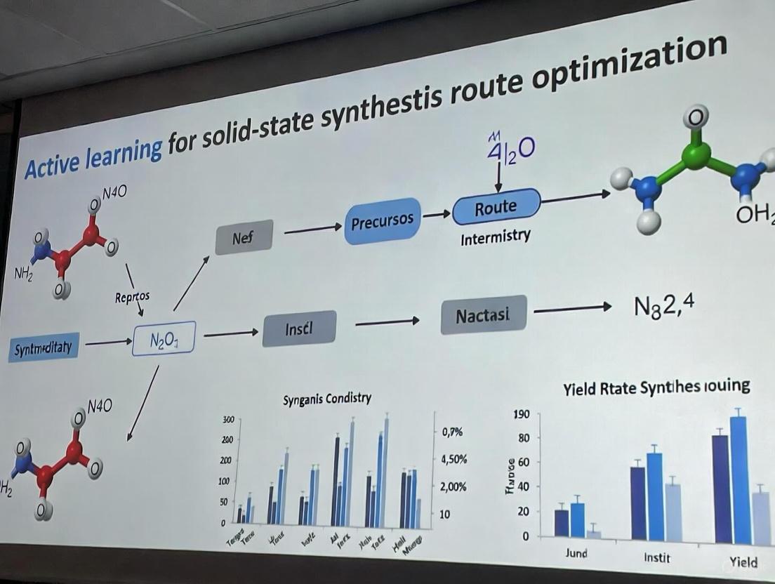
Active Learning for Solid-State Synthesis: AI-Driven Route Optimization in Materials Science and Drug Development

Abstract

This article explores the transformative role of active learning (AL), a subfield of artificial intelligence, in optimizing solid-state synthesis routes—a critical challenge in materials science and drug development. It covers the foundational principles of AL, which iteratively guides experiments to maximize information gain, and details its methodological implementation in autonomous laboratories. The content addresses common troubleshooting and optimization challenges, provides a comparative validation of various AL strategies against traditional methods, and highlights real-world successes, such as the A-Lab's demonstration of synthesizing 41 new inorganic materials. Aimed at researchers and scientists, this review underscores how AL accelerates the discovery of high-performance materials while significantly reducing experimental time and costs.

What is Active Learning? Foundations for Solid-State Synthesis

Core Concepts and Definitions

Active Learning (AL) represents a paradigm shift in scientific experimentation, moving from traditional passive data collection to an intelligent, iterative process where the learning algorithm itself selects the most informative data points to be labeled or experiments to be performed. This data-centric approach is designed to maximize model performance or knowledge gain while minimizing the often prohibitive cost of experimental synthesis and characterization [1].

Within the context of solid-state synthesis and materials discovery, AL functions as a closed-loop system. This system integrates computational prediction, robotic experimentation, and data analysis to accelerate the identification and optimization of novel materials [2]. The core principle involves using an agent—often a machine learning model—to decide which experiment to conduct next based on the data collected from all previous experiments. This is in stark contrast to one-time, static design-of-experiments or high-throughput screening that lacks a sequential decision-making component.

The fundamental components of an AL cycle are:

• Proxy Model: A surrogate model that predicts material properties or synthesis outcomes.
• Acquisition Function: A strategy that uses the model's state to quantify the potential value of any new experiment.
• Experimental Oracle: The automated or robotic system that executes the proposed experiment and returns results (e.g., yield, phase purity).
• Update Rule: The procedure for incorporating new data into the model to refine future predictions.

This methodology is particularly critical in fields like materials science and drug development, where the synthesis and characterization of a single sample can require extensive resources, expert knowledge, and time [1]. By intelligently selecting which experiments to run, AL can dramatically reduce the number of experiments required to achieve a research objective, such as discovering a new battery material or optimizing a catalytic reaction.

Foundational Principles and Algorithmic Strategies

Active learning strategies are grounded in several core principles, which are implemented through specific acquisition functions. The table below summarizes the primary principles and their corresponding algorithmic strategies used in AL for scientific domains.

Table 1: Foundational Principles and Corresponding Active Learning Strategies

Principle	Description	Example AL Strategies
Uncertainty Estimation	Selects samples where the model's prediction is most uncertain, aiming to reduce model variance and improve overall accuracy.	Least Confidence Margin (LCMD), Tree-based Uncertainty (Tree-based-R) [1].
Diversity	Aims to select a set of data points that are representative of the entire input space, ensuring the model learns from a broad range of conditions.	Geometry-based (GSx), Euclidean Distance-based (EGAL) [1].
Expected Model Change	Selects samples that are expected to cause the greatest change in the current model, thereby accelerating learning.	Expected Model Change Maximization (EMCM) [1].
Representativeness	Selects samples that are similar to many other unlabeled points, ensuring the model learns from common scenarios.	Representative-Diversity hybrids (RD-GS) [1].
Hybrid Strategies	Combines multiple principles (e.g., uncertainty and diversity) to balance exploration of the unknown with refinement of known areas.	RD-GS (Representativeness-Diversity) [1].

In practice, the choice of strategy depends heavily on the specific task and data characteristics. Benchmark studies have shown that in the early, data-scarce phase of a project, uncertainty-driven and diversity-hybrid strategies (like RD-GS) clearly outperform random sampling and geometry-only heuristics [1]. As the volume of labeled data increases, the performance advantage of specialized AL strategies tends to diminish, with all methods converging toward similar model accuracy.

Experimental Protocols: Implementation in a Self-Driving Lab

The following protocol details the implementation of an active learning cycle within an autonomous laboratory for solid-state synthesis, based on the landmark A-Lab system [3].

Protocol: Autonomous Synthesis and Optimization of Novel Inorganic Materials

Objective: To autonomously synthesize a target inorganic material predicted to be stable by computational screening, and to iteratively optimize the synthesis recipe to maximize target yield.

Primary Materials and Instruments: Table 2: Research Reagent Solutions and Essential Materials for Solid-State Synthesis

Item Name	Function/Description
Precursor Powders	High-purity solid powders of constituent elements or simple compounds. Serve as the starting materials for solid-state reactions.
Alumina Crucibles	Containers for holding powder mixtures during high-temperature heating. They are inert and withstand repeated heating cycles.
Box Furnaces	Provide controlled high-temperature environments necessary for solid-state synthesis reactions to occur.
Robotic Milling Apparatus	Automates the grinding and mixing of precursor powders to ensure homogeneity and improve reactivity.
X-ray Diffractometer (XRD)	The primary characterization tool used to identify crystalline phases present in the synthesis product and estimate their weight fractions.

Methodology:

• Target Identification and Initial Recipe Proposal:

  • Input: A set of novel, computationally-predicted stable materials are identified from ab initio databases (e.g., Materials Project, Google DeepMind) [3].
  • Action: For each target material, an AI model trained on historical literature data using natural-language processing proposes up to five initial solid-state synthesis recipes. These recipes are based on chemical analogy to known materials [2] [3].
  • Output: A set of proposed recipes specifying precursor powders and an initial synthesis temperature.

• Robotic Synthesis Execution:

  • A robotic arm transfers weighed precursor powders into a mixing vessel.
  • An automated system mills the powders to create a homogeneous mixture.
  • The mixture is transferred into an alumina crucible.
  • A second robotic arm loads the crucible into one of four box furnaces for heating according to the proposed time-temperature profile [3].

• Automated Product Characterization and Analysis:

  • After cooling, the sample is automatically transferred to a grinding station and prepared for analysis.
  • The sample is analyzed via X-ray Diffraction (XRD).
  • The XRD pattern is interpreted by a ensemble of machine learning models trained on experimental structures, which identify the crystalline phases present [3].
  • The phase identification is confirmed and quantified via automated Rietveld refinement. The weight fraction of the target material is calculated and reported.

• Active Learning-Driven Iteration:

  • Decision Point: If the target yield exceeds a pre-defined threshold (e.g., >50%), the process is deemed successful. If not, the AL loop is initiated [3].
  • Algorithm: The Autonomous Reaction Route Optimization with Solid-State Synthesis (ARROWS³) algorithm is employed. This active learning system integrates ab initio computed reaction energies with the observed experimental outcomes [3].
  • Hypothesis Generation: ARROWS³ uses two key hypotheses to propose a new, improved recipe: a. It prioritizes reaction pathways that avoid intermediate phases with a low thermodynamic driving force (<50 meV per atom) to form the final target, as these can lead to kinetic traps [3]. b. It leverages a growing database of observed pairwise solid-state reactions to infer reaction pathways and prune the search space of possible recipes, avoiding redundant experiments [3].
  • The newly proposed recipe is executed (return to Step 2), and the loop continues until the target is synthesized or all plausible recipes are exhausted.

Active Learning Cycle for Solid-State Synthesis

Quantitative Comparison of Active Learning Strategies

The effectiveness of different AL strategies can be quantitatively benchmarked, particularly when integrated with Automated Machine Learning (AutoML) frameworks that dynamically select and tune model types. The following data, derived from a comprehensive benchmark study on materials science regression tasks, compares the performance of various strategies in a small-data regime [1].

Table 3: Benchmarking of Active Learning Strategies with AutoML on Materials Datasets

Strategy Type	Example Strategies	Early-Stage Performance (Data-Scarce)	Late-Stage Performance (Data-Rich)	Key Characteristics
Uncertainty-Driven	LCMD, Tree-based-R	Clearly outperforms random sampling	Converges with other methods	Selects points where model is most uncertain, rapidly improving accuracy.
Diversity-Hybrid	RD-GS	Clearly outperforms random sampling	Converges with other methods	Balances exploration of input space with representativeness.
Geometry-Only	GSx, EGAL	Performance closer to baseline	Converges with other methods	Focuses on spatial coverage of the feature space.
Baseline	Random-Sampling	Reference for comparison	Reference for comparison	Selects experiments randomly, lacking intelligent selection.

Key Insight: The benchmark demonstrates that the choice of AL strategy is most critical during the early stages of an experimental campaign. Uncertainty-based and hybrid methods can rapidly steer the model toward high performance with fewer data points, leading to significant resource savings [1]. This underscores the importance of strategic experiment selection in resource-constrained environments like solid-state synthesis.

Advanced Architectures and Implementation Guidelines

The Role of Large Language Models (LLMs) as Cognitive Agents

Recent advances have introduced hierarchical, multi-agent systems powered by Large Language Models (LLMs) as the "brain" of autonomous laboratories. Frameworks like ChemAgents utilize a central task manager that coordinates role-specific agents (e.g., Literature Reader, Experiment Designer, Robot Operator) to conduct on-demand chemical research [2]. Similarly, Coscientist is an LLM-driven system capable of autonomously designing, planning, and executing complex chemical experiments by leveraging tool-use capabilities such as web searching, document retrieval, and code-based control of robotic systems [2]. These systems mark a significant step towards generalist autonomous research platforms.

Key Constraints and Mitigation Strategies

Despite their promise, autonomous laboratories face several constraints that must be addressed for widespread adoption [2]:

• Data Quality and Scarcity: AI model performance is heavily dependent on high-quality, diverse data. Noisy or scarce experimental data can hinder accurate predictions.
  • Mitigation: Develop standardized data formats, utilize high-quality simulation data, and employ uncertainty analysis.
• Model Generalization: Most AI models are highly specialized and struggle to generalize across different reaction types or material systems.
  • Mitigation: Train foundation models across different domains and use transfer learning to adapt to new data.
• LLM Reliability: LLMs can generate plausible but incorrect information ("hallucinations") without indicating uncertainty, potentially leading to failed experiments.
  • Mitigation: Implement targeted human oversight and robust fact-checking mechanisms within the agent workflow.
• Hardware Integration: A lack of modular hardware architectures makes it difficult to reconfigure platforms for different chemical tasks.
  • Mitigation: Develop standardized interfaces and extend mobile robotic capabilities to include specialized analytical modules.

Hierarchical Multi-Agent System for Autonomous Research

Active learning (AL) represents a paradigm shift in scientific experimentation, moving from traditional high-throughput screening to an intelligent, data-efficient approach that accelerates discovery while minimizing resource consumption. In the context of solid-state synthesis and materials science, AL addresses a critical bottleneck: the prohibitive cost and time required for experimental synthesis and characterization [4]. This methodology is particularly valuable for optimizing solid-state synthesis routes, where each experimental cycle can require expert knowledge, expensive equipment, and days of processing [3]. By integrating surrogate models, acquisition functions, and experimental validation into a closed-loop system, active learning enables researchers to navigate complex experimental spaces systematically, prioritizing the most promising experiments based on iterative model predictions [2].

The fundamental active learning cycle operates through three interconnected components: surrogate models that approximate complex physical systems, acquisition functions that quantify the potential value of new experiments, and experimental validation that grounds the process in empirical reality. This framework has demonstrated remarkable success in practical applications. For instance, in autonomous materials discovery platforms, active learning has achieved order-of-magnitude efficiency gains over traditional approaches, successfully synthesizing novel compounds with minimal human intervention [4] [3]. Similarly, in computational physiology, AL has reduced the computational costs of inverse parameter identification by strategically selecting training data for surrogate models [5].

Core Component 1: Surrogate Models

Definition and Purpose

Surrogate models, also known as metamodels or reduced-order models, are computationally efficient approximations of complex, high-fidelity simulation models or experimental processes. They serve as replacement models during the iterative optimization phases of active learning, where executing the full model repeatedly would be prohibitively expensive [5]. In solid-state synthesis optimization, surrogate models learn the relationship between synthesis parameters (e.g., precursor selection, temperature profiles, processing conditions) and experimental outcomes (e.g., phase purity, yield, material properties) [4]. By capturing the essential input-output relationships of the actual experimental process, these models enable rapid exploration of the synthesis parameter space while dramatically reducing the need for physical experiments.

The primary advantage of surrogate models lies in their computational efficiency. Once trained, they can generate predictions in seconds or milliseconds compared to hours or days for actual experiments or high-fidelity simulations. This speed advantage makes them ideal for active learning cycles that require numerous iterations to converge on optimal solutions [5]. For example, in biomechanical parameter identification, neural network surrogates have achieved speed improvements of several orders of magnitude compared to finite element simulations while maintaining high accuracy in predicting material behavior [5].

Model Selection and Implementation

Different surrogate model architectures offer distinct advantages depending on the nature of the modeling task:

• Recurrent Neural Networks (RNNs) are particularly effective for modeling time-dependent processes such as viscoelastic material behavior or kinetic processes in solid-state reactions. Their ability to maintain a persistent state makes them analogous to internal variables in constitutive models [5].
• Feed-Forward Neural Networks excel at capturing nonlinear static relationships, such as mapping material composition to final properties in hyperelastic metamodels [5].
• Gaussian Process Regression provides natural uncertainty quantification alongside predictions, making them valuable for Bayesian optimization approaches where uncertainty estimates guide exploration [5].
• Graph Neural Networks and Transformers have recently achieved unprecedented accuracy in predicting material properties across diverse chemical spaces, particularly when dealing with structured representations of materials [4].

The process for developing effective surrogate models begins with generating an initial training dataset using space-filling designs such as Latin Hypercube Sampling or Poisson's disk sampling to ensure good coverage of the parameter space [5]. The model is then trained to minimize the difference between its predictions and the outputs from high-fidelity simulations or experiments. For dynamic processes, sequence-based loss functions that account for temporal evolution are typically employed [5].

Application in Solid-State Synthesis

In solid-state synthesis optimization, surrogate models can predict the outcome of proposed synthesis routes before physical execution. For instance, machine learning interatomic potentials have enabled microsecond-scale molecular dynamics simulations at near-density functional theory accuracy, revealing non-Arrhenius transport behavior and overturning established transport mechanisms [4]. These models learn from both computational data and experimental results, creating a compressed representation of the complex relationship between synthesis parameters and material outcomes.

Recent advances have integrated surrogate models with automated machine learning (AutoML) systems that automatically search and optimize between different model families and their hyperparameters [1]. This approach is particularly valuable in materials science, where experimentation and characterization are resource-intensive, making large-scale manual model tuning impractical. AutoML has been proven to be an excellent tool for material design, automatically selecting the optimal surrogate model architecture for specific synthesis prediction tasks [1].

Core Component 2: Acquisition Functions

Role in Active Learning

Acquisition functions form the decision-making engine of the active learning loop, quantitatively evaluating which experiments or simulations would provide the maximum information gain if performed next. These functions serve as mathematical heuristics that balance the competing objectives of exploration (sampling from regions of high uncertainty) and exploitation (refining knowledge in promising regions) [1]. In solid-state synthesis optimization, acquisition functions analyze the predictions of surrogate models to identify the most "rewarding" synthesis conditions to test experimentally, thereby maximizing the efficiency of the experimental campaign [5].

The importance of well-designed acquisition functions cannot be overstated—they directly determine the data efficiency of the entire active learning process. Empirical studies have demonstrated that effective acquisition strategies can reduce the number of experiments required to reach a target level of performance by 60-70% compared to random sampling [1] [3]. For example, in alloy design and ternary phase-diagram regression, uncertainty-driven active learning has achieved state-of-the-art accuracy using only 30% of the data typically required by traditional approaches [1].

Classification and Comparison

Acquisition functions can be categorized based on their underlying mathematical principles:

Table 1: Classification of Acquisition Functions for Regression Tasks

Category	Principle	Representative Methods	Strengths	Limitations
Uncertainty-Based	Selects points where model prediction uncertainty is highest	Monte Carlo Dropout [5], Query-by-Committee [5]	Directly reduces model uncertainty; Simple to implement	May overlook data distribution structure
Diversity-Based	Maximizes coverage of the input feature space	RD-GS [1]	Ensures representative sampling; Avoids redundancy	Ignores model uncertainty; May sample unimportant regions
Expected Model Change	Selects points that would most alter the current model	EMCM [1]	Focuses on model improvement; Efficient for complex models	Computationally intensive for large datasets
Hybrid Approaches	Combines multiple principles for balanced sampling	LCMD, Tree-based-R [1]	Balances exploration and exploitation; Robust performance	More complex to implement and tune

Performance Benchmarking

Recent comprehensive benchmarking studies have evaluated various acquisition functions in materials science regression tasks. These studies reveal that the relative performance of different strategies depends significantly on the stage of the active learning process and the specific characteristics of the dataset:

Table 2: Performance Comparison of Acquisition Functions in Materials Science Regression [1]

Strategy Type	Early-Stage Performance	Late-Stage Performance	Consistency Across Datasets	Computational Overhead
Uncertainty-Driven (LCMD)	High	Medium	High	Low
Diversity-Hybrid (RD-GS)	High	Medium	Medium	Medium
Tree-Based (Tree-based-R)	High	High	High	Low
Geometry-Only (GSx, EGAL)	Low	Medium	Low	Low
Random Sampling	Low	Medium	High	Very Low

Benchmark results indicate that early in the acquisition process when labeled data is scarce, uncertainty-driven and diversity-hybrid strategies clearly outperform geometry-only heuristics and random sampling [1]. These methods excel at selecting informative samples that rapidly improve model accuracy. However, as the labeled set grows, the performance gap narrows and all methods eventually converge, indicating diminishing returns from active learning under AutoML frameworks [1].

Interestingly, despite the development of sophisticated acquisition functions, empirical studies have found that in general settings, no single-model approach consistently outperforms entropy-based strategies [6]. This surprising result serves as a reality check for the field, suggesting that simple, well-understood acquisition functions may provide more robust performance across diverse applications than increasingly complex alternatives.

Core Component 3: Experimental Validation

Closing the Loop

Experimental validation represents the critical ground-truthing step that closes the active learning loop, transforming it from a computational exercise into a scientifically rigorous process. This phase involves executing the experiments selected by the acquisition function and measuring their outcomes to generate new labeled data points [3]. In solid-state synthesis, this typically entails robotic execution of proposed synthesis recipes followed by automated characterization of the resulting products [2]. The validation data serves dual purposes: it provides training examples to improve the surrogate model in subsequent iterations, and it progressively converges toward optimal synthesis conditions.

The importance of robust experimental validation cannot be overstated, as it ensures that the active learning process remains anchored in physical reality rather than diverging into computationally plausible but experimentally invalid regions of the parameter space. Autonomous laboratories like the A-Lab have demonstrated the power of tight integration between computational prediction and experimental validation, successfully synthesizing 41 of 58 novel target compounds through iterative optimization [3]. Their success rate of 71% underscores the effectiveness of this approach for accelerating materials discovery.

Validation Methodologies

Different experimental domains employ specialized validation techniques appropriate for their specific measurement requirements:

• Solid-State Synthesis: Automated platforms like the A-Lab utilize robotic arms for sample preparation, transfer of precursors to crucibles, loading into box furnaces for heating, and subsequent grinding of products into fine powders for X-ray diffraction (XRD) analysis [3]. Phase identification and weight fractions are extracted from XRD patterns using probabilistic machine learning models trained on experimental structures, with confirmation through automated Rietveld refinement [3].

• Biomechanical Parameter Identification: Experimental validation involves mechanical testing of material specimens under controlled deformation conditions while recording force responses. For inhomogeneous deformation states, digital image correlation techniques may be employed to capture full-field displacement data [5].

• Chemical Synthesis: Automated platforms integrate robotic liquid handling systems with analytical instrumentation such as ultra-performance liquid chromatography-mass spectrometry (UPLC-MS) and benchtop nuclear magnetic resonance (NMR) spectroscopy [2]. Heuristic decision makers process orthogonal analytical data to mimic expert judgments, using techniques like dynamic time warping to detect reaction-induced spectral changes [2].

A critical aspect of experimental validation is handling failed syntheses and unexpected outcomes. Rather than considering these as mere failures, sophisticated active learning systems analyze them to extract valuable information about synthesis barriers. Common failure modes in solid-state synthesis include slow reaction kinetics, precursor volatility, amorphization, and computational inaccuracies in phase stability predictions [3]. Documenting and learning from these failures provides direct and actionable suggestions for improving both computational screening techniques and synthesis design strategies.

Integrated Workflow and Protocols

Standard Operating Procedure

Implementing an effective active learning loop for solid-state synthesis optimization requires careful integration of the three core components into a seamless workflow. The following protocol outlines a standardized approach based on successful implementations in autonomous materials discovery platforms:

Phase 1: Initialization

• Define Target: Identify the target material to be synthesized, ensuring it is predicted to be thermodynamically stable or nearly stable (within <10 meV/atom of the convex hull) based on ab initio computations [3].
• Establish Baseline: Generate initial synthesis recipes using literature-inspired approaches, such as natural language processing models trained on historical synthesis data [3].
• Characterization Setup: Configure automated characterization instruments (e.g., XRD, spectroscopy) and validate measurement protocols using standard reference materials.

Phase 2: Active Learning Cycle

• Surrogate Model Training: Train the selected surrogate model architecture on all available labeled data (both initial and accumulated from previous cycles).
• Candidate Generation: Use the trained surrogate model to predict outcomes for a large pool of candidate synthesis conditions within the predefined parameter space.
• Acquisition Function Evaluation: Apply the selected acquisition function to rank candidate experiments by their expected information gain or potential improvement.
• Experimental Execution: Robotically execute the top-ranked synthesis recipes, including precursor dispensing, mixing, heating according to specified profiles, and product handling [3].
• Automated Characterization: Perform structural and compositional analysis of synthesis products using integrated characterization tools.
• Data Integration: Extract phase identification and yield information from characterization data and add the newly labeled examples to the training dataset [3].

Phase 3: Termination and Analysis

• Convergence Check: Evaluate if stopping criteria have been met (e.g., target yield >50%, diminishing returns, or budget exhaustion).
• Result Validation: Perform additional characterization on optimized materials to confirm properties beyond phase purity.
• Knowledge Extraction: Analyze the accumulated data to extract insights about synthesis-structure-property relationships for future campaigns.

The following workflow diagram illustrates the integrated active learning process for solid-state synthesis optimization:

Implementing an active learning system for solid-state synthesis requires both computational and experimental resources:

Table 3: Essential Research Reagents and Resources for Active Learning-Driven Synthesis

Resource Category	Specific Examples	Function in AL Workflow	Implementation Considerations
Computational Databases	Materials Project [3], Google DeepMind stability data [3]	Provides initial target screening and thermodynamic references	Ensure air-stability predictions for targets; Cross-reference multiple databases
Precursor Materials	High-purity oxide and phosphate powders [3]	Raw materials for solid-state synthesis	Characterize particle size, purity, and moisture content before use
Robotic Automation	Robotic arms for powder handling [3], Mobile sample transport robots [2]	Executes synthesis recipes with minimal human intervention	Implement collision avoidance and error recovery protocols
Heating Systems	Programmable box furnaces [3]	Performs solid-state reactions at controlled temperatures	Calibrate temperature profiles and monitor thermal uniformity
Characterization Instruments	X-ray diffractometers [3], UPLC-MS [2], Benchtop NMR [2]	Provides phase identification and yield quantification	Automate data analysis with ML models for real-time feedback
Surrogate Model Platforms	Bayesian optimization frameworks [5], AutoML systems [1]	Accelerates parameter space exploration	Select models appropriate for data type (RNN for kinetics, etc.)
Acquisition Functions	Uncertainty sampling [5], Diversity methods [1], Hybrid approaches [1]	Guides experiment selection	Balance exploration vs. exploitation based on campaign stage

Case Study: A-Lab Implementation

The A-Lab autonomous materials discovery platform provides a compelling case study of the integrated active learning framework applied to solid-state synthesis optimization. Over 17 days of continuous operation, the A-Lab successfully synthesized 41 of 58 novel target compounds identified using large-scale ab initio phase-stability data [3]. This 71% success rate demonstrates the practical effectiveness of combining surrogate models, acquisition functions, and robotic validation.

The A-Lab implementation featured several innovative elements. For surrogate modeling, the system utilized multiple complementary approaches: natural-language models trained on literature data for initial recipe generation, and thermodynamic models informed by ab initio computations for active learning optimization [3]. The acquisition function employed a sophisticated strategy called ARROWS3 (Autonomous Reaction Route Optimization with Solid-State Synthesis), which integrated observed synthesis outcomes with computed reaction energies to predict optimal solid-state reaction pathways [3].

A key insight from the A-Lab implementation was the importance of handling failed syntheses as learning opportunities rather than mere failures. Analysis of the 17 unobtained targets revealed specific failure modes including slow reaction kinetics, precursor volatility, amorphization, and computational inaccuracies [3]. This analysis provided direct, actionable suggestions for improving both computational screening techniques and synthesis design strategies, highlighting that minor adjustments to the lab's decision-making algorithm could increase the success rate to 74%, with further improvements to 78% possible with enhanced computational techniques [3].

The following diagram illustrates the specific active learning workflow implemented in the A-Lab platform:

The integration of surrogate models, acquisition functions, and experimental validation represents a powerful framework for accelerating scientific discovery in solid-state synthesis and related fields. Current research directions focus on addressing several key challenges to further enhance the capabilities of active learning systems.

For surrogate models, emerging approaches include physics-informed neural networks that incorporate known physical constraints and conservation laws directly into the model architecture, improving extrapolation accuracy and data efficiency [4]. Transfer learning techniques are being developed to leverage knowledge from data-rich chemical domains to accelerate learning in data-scarce environments, particularly for multivalent systems where experimental data is limited [4]. For acquisition functions, recent benchmarks highlight the need for more robust evaluation methodologies that account for real-world constraints like batch parallelism and multi-fidelity data sources [6] [1].

The most significant advances are likely to come from improved integration of the three core components. Autonomous laboratories are increasingly adopting hierarchical multi-agent systems where different components specialize in specific tasks yet coordinate through a central planner [2]. For example, the ChemAgents framework features a central Task Manager that coordinates four role-specific agents (Literature Reader, Experiment Designer, Computation Performer, and Robot Operator) for on-demand autonomous chemical research [2]. Such architectures promise more robust and adaptable systems capable of handling the complex, multi-step decision-making required for real scientific discovery.

In conclusion, the core components of active learning—surrogate models, acquisition functions, and experimental validation—form a powerful framework for accelerating materials discovery and optimization. When thoughtfully integrated into a closed-loop system, these components enable researchers to navigate complex experimental spaces with unprecedented efficiency, as demonstrated by successful implementations in autonomous laboratories. As these technologies continue to mature, they promise to transform the pace and scope of scientific discovery across chemistry, materials science, and related fields.

The discovery and optimization of materials through solid-state synthesis are fundamentally constrained by the immense, high-dimensional space of possible experimental parameters. This space encompasses variations in chemistry, crystal structure, processing conditions, and microstructure [7]. The traditional approach of relying on trial-and-error or even high-throughput methods that attempt to densely populate this entire phase space is often impractical, time-consuming, and resource-intensive [7]. The central challenge is to efficiently guide experiments towards materials with desired properties without exhaustively testing every possible combination.

Active learning (AL), a paradigm from the fields of machine learning and statistical experimental design, offers a powerful solution to this challenge. It provides a systematic, iterative framework for making optimal decisions about which experiment to perform next. The core of this approach is an active learning loop: a surrogate model makes predictions about the material property of interest; these predictions, together with their associated uncertainties, are fed into a utility function (also called an acquisition function); the optimal point of this utility function dictates the next experiment or calculation to be performed [7]. The results of this experiment then augment the training data, and the loop continues until the target performance is met, dramatically reducing the number of experiments required.

Active Learning Methodologies and Experimental Protocols

The following section details the core components for implementing an active learning strategy in a solid-state synthesis workflow.

The Active Learning Workflow for Synthesis Optimization

The active learning process for optimizing solid-state synthesis can be visualized as a cyclic workflow, where computational guidance and experimental validation are tightly integrated. This workflow is designed to efficiently navigate the parameter space by strategically selecting the most informative experiments.

Core Components of the Active Learning Protocol

Surrogate Models and Utility Functions

The surrogate model, often a machine learning regression model, learns the relationship between synthesis parameters and the target material property from the available data. In parallel, the model estimates the uncertainty of its predictions for unexplored parameter combinations. The choice of utility function is critical as it balances the exploration of uncertain regions with the exploitation of known high-performing regions [7]. Common functions include:

• Expected Improvement (EI): Selects points that offer the highest potential improvement over the current best observation [7].
• Upper Confidence Bound (UCB): Selects points based on a weighted sum of the predicted mean and its uncertainty.
• Density-Aware Methods: Recent advances, such as Density-Aware Greedy Sampling (DAGS), integrate data density with uncertainty estimation. This is particularly effective for large design spaces, as it prevents the sampling of outliers and focuses on the most promising, densely populated regions of the parameter space [8].

Queue Prioritization for Generative Workflows

In workflows that use generative AI to propose new candidate materials, an additional step of queue prioritization can be integrated. A dedicated active learning model can be used to score and rank the AI-generated candidates, ensuring that the most promising ones are synthesized and tested first. This prevents the workflow from expending resources on nonsensical or low-quality candidates and can significantly increase the number of high-performing candidates identified—in one case study, increasing the average from 281 to 604 out of 1000 novel candidates [9].

Detailed Experimental Protocol: A Case Study in Wollastonite Synthesis

The following protocol is inspired by a recent study on the single-step solid-state synthesis of Wollastonite-2M using rice husk ash (RHA), adapted here within an active learning framework [10].

Application Note: Optimizing the synthesis of single-phase Wollastonite-2M from RHA and natural limestone. Targeted Property: Phase purity (minimization of secondary crystalline phases as determined by X-ray Diffraction).

Initial Dataset Creation:

• Define Parameter Ranges: Based on literature, define the initial search space.
• Design of Experiments (DoE): Use a space-filling design (e.g., Latin Hypercube Sampling) to select 10-15 initial (sintering temperature, sintering time, CaO:SiO₂ molar ratio) triplets from the predefined ranges.
• Initial Experimentation: Execute the synthesis and characterization for each initial data point.

Active Learning Loop:

• Model Training: Train a Gaussian Process Regression (GPR) model on the current dataset. The GPR is ideal as it provides inherent uncertainty estimates.
• Candidate Selection: Using the GPR model, predict the phase purity and uncertainty for a large number of candidate parameter sets within the search space. Calculate the Expected Improvement for each candidate.
• Next Experiment: Select the candidate parameter set with the highest Expected Improvement.
• Synthesis Execution:
  • Mixing: Grind the RHA (source of SiO₂) and limestone (CaCO₃, source of CaO) in the selected molar ratio (e.g., ~1:1) using a ball mill for 30 minutes.
  • Pelletizing: Press the homogeneous powder mixture into pellets under uniaxial pressure.
  • Sintering: Heat the pellets in a furnace at the selected temperature (e.g., 1150-1350°C) for the selected duration (e.g., 2-8 hours), followed by free cooling in the air [10].
• Characterization: Analyze the synthesized product using X-ray Powder Diffraction (XRD) to determine the phase composition and quantify the primary phase purity.
• Data Augmentation: Add the new (parameters, purity) data pair to the training dataset.
• Iteration: Repeat steps 1-6 until a predefined purity threshold is achieved or the experimental budget is exhausted.

Quantitative Data and Research Reagent Solutions

Synthesis Parameter Space and Performance Metrics

The optimization of solid-state synthesis involves navigating a multi-dimensional space of continuous and discrete parameters. The table below summarizes the key parameters, their typical ranges based on the wollastonite case study and general synthesis principles, and the target properties that can be optimized [10].

Table 1: Key Parameters and Target Properties in Solid-State Synthesis Optimization

Parameter Category	Specific Parameter	Typical Range / Options	Measurable Target Property
Thermal Profile	Sintering Temperature	1150 - 1350 °C [10]	Phase Purity (from XRD)
	Sintering Time	2 - 8 hours [10]	Crystallite Size (from XRD Scherrer)
	Heating/Cooling Rate	1 - 10 °C/min	Particle Morphology (from SEM)
Stoichiometry	CaO:SiO₂ Molar Ratio	0.9:1 - 1.1:1	Lattice Parameters (from XRD Rietveld)
	Dopant/Additive Concentration	0 - 5 mol%	Bulk Density/Porosity
Processing	Grinding Time	15 - 60 minutes	Target Functional Property (e.g., CO₂ uptake)
	Applied Pressure (for pellets)	10 - 50 MPa

Research Reagent Solutions for Solid-State Synthesis

The following table lists essential materials and equipment required for setting up an active learning-driven solid-state synthesis laboratory, with a focus on the wollastonite case study.

Table 2: Essential Research Reagent Solutions for Solid-State Synthesis

Item Name	Function / Application	Specific Example / Note
Rice Husk Ash (RHA)	Eco-friendly, high-purity (≈90% SiO₂) silica source for silicate synthesis. Reduces costs and utilizes agricultural waste [10].	Should be characterized for SiO₂ content and impurities before use.
Calcium Carbonate (CaCO₃)	Common precursor for introducing CaO into the reaction.	High-purity powder; can be replaced by calcium hydrate.
Planetary Ball Mill	Provides mechanical energy for homogenizing and reducing particle size of precursor mixtures, critical for reaction kinetics.	Milling time and speed are optimizable parameters.
High-Temperature Furnace	Provides the thermal energy required for solid-state diffusion and reaction to form the target crystalline phase.	Must be capable of reaching temperatures up to 1400-1500°C with precise control.
Uniaxial Press	Forms powder mixtures into dense pellets, increasing inter-particle contact and improving reaction yield.	Applied pressure is an optimizable processing parameter.
X-ray Diffractometer (XRD)	The primary characterization tool for verifying phase formation, quantifying purity, and determining crystal structure.	Essential for generating the target property data (e.g., phase purity) for the active learning model.

The integration of active learning into solid-state synthesis represents a paradigm shift from empirically guided exploration to a principled, data-driven decision-making process. By leveraging surrogate models and utility functions to strategically select the most informative experiments, researchers can dramatically compress the time and resources required to discover and optimize new materials. The detailed workflow, protocols, and resource guides provided here offer a practical roadmap for implementing this powerful approach, turning the critical challenge of navigating vast parameter spaces into a manageable and efficient scientific endeavor.

Active Learning (AL) has emerged as a transformative paradigm in scientific research, strategically overcoming the inefficiencies of traditional trial-and-error and the high costs associated with exhaustive high-throughput screening (HTS). By integrating artificial intelligence (AI) with robotic experimentation, AL creates a closed-loop system that iteratively selects the most informative experiments, dramatically accelerating the discovery and optimization of novel materials and drug molecules [2] [11]. This approach is particularly powerful in solid-state synthesis and drug discovery, where it leverages machine learning models to guide experimental planning, execution, and analysis with minimal human intervention. This Application Note details the quantitative benefits of AL, provides executable protocols for its implementation, and visualizes its core workflows, framing these advances within the context of solid-state synthesis route optimization.

Quantitative Advantages of Active Learning

The following tables summarize performance data from recent, high-impact studies applying Active Learning across chemical and materials domains.

Table 1: Performance of Active Learning in Materials and Molecule Discovery

Application Area	System / Method	Key Performance Metric	Result
Solid-State Materials Discovery	A-Lab [3]	Novel materials synthesized successfully	41 out of 58 targets (71% success rate)
		Duration of continuous operation	17 days
Molecular Potency Optimization	ActiveDelta (99 datasets) [12]	Identification of more potent & diverse inhibitors	Outperformed standard exploitative AL
Virtual Screening Acceleration	Bayesian Optimization (100M library) [13]	Top ligands identified after screening	94.8% of top-50k found after testing 2.4% of library
De Novo Drug Design	GM with AL (CDK2 target) [14]	Experimentally confirmed active molecules	8 out of 9 synthesized molecules showed activity

Table 2: Active Learning Methods and Their Applications

AL Method / Architecture	Domain	Key Advantage
ActiveDelta (Paired Representation) [12]	Drug Discovery	Excels in low-data regimes; identifies more diverse inhibitors
ARROWS3 [3]	Solid-State Synthesis	Uses active learning grounded in thermodynamics to optimize synthesis routes
Bayesian Optimization (D-MPNN) [13]	Virtual Screening	Massive reduction in computational cost for docking massive libraries
Nested AL Cycles (VAE-based) [14]	De Novo Drug Design	Integrates generative AI with physics-based oracles for target engagement
Deep Batch AL (COVDROP/COVLAP) [15]	ADMET & Affinity Prediction	Maximizes joint entropy for batch diversity and model performance

Application Note: The A-Lab for Solid-State Synthesis

The A-Lab represents a landmark implementation of AL for autonomous solid-state synthesis, demonstrating a closed-loop workflow from computational target identification to synthesized material [3].

Workflow and Protocol

The A-Lab's operation is a continuous cycle of planning, execution, and learning. The following diagram illustrates this integrated workflow.

Detailed Experimental Protocol

Objective: To autonomously synthesize and optimize a novel, computationally predicted inorganic material.

Starting Requirements:

• Computational Targets: A set of air-stable, theoretically stable inorganic materials identified from the Materials Project or similar ab initio databases [3].
• Hardware: Integrated robotic station with powder handling capabilities, box furnaces for solid-state reactions, and an X-ray Diffractometer (XRD).
• Software & Data: AI models trained on historical synthesis literature, ML models for XRD phase identification, and an active learning algorithm (e.g., ARROWS3).

Procedure:

• Target Input: Provide the A-Lab with the chemical formula of a target material predicted to be stable.
• Initial Recipe Proposal:
  • A natural-language processing model analyzes historical data to propose initial solid-state synthesis recipes based on precursor analogy [3].
  • A second ML model recommends an initial synthesis temperature.
• Robotic Execution:
  • The robotic system automatically dispenses, weighs, and mixes precursor powders in an alumina crucible [3].
  • A robotic arm transfers the crucible to a box furnace for heating under prescribed conditions (temperature, time, atmosphere).
• Product Characterization & Analysis:
  • After cooling, the sample is automatically ground and transferred for XRD analysis.
  • A convolutional neural network analyzes the XRD pattern to identify crystalline phases and estimate weight fractions [2] [3].
  • Results are validated with automated Rietveld refinement.
• Active Learning Cycle:
  • Decision Point: If the target yield is >50%, the experiment is concluded successfully.
  • If yield is <50%: The ARROWS3 active learning algorithm is triggered.
  • ARROWS3 integrates the observed reaction pathway (e.g., intermediate phases) with thermodynamic data from the Materials Project.
  • The algorithm prioritizes new precursor sets or conditions that avoid low-driving-force intermediates, proposing a new recipe with a higher probability of success [3].
• Iteration: Steps 3-5 are repeated until either the target is successfully synthesized or a predefined number of recipe attempts are exhausted.

Application Note: Active Learning in Drug Discovery

AL has proven highly effective in various drug discovery stages, from virtual screening to hit optimization.

Workflow for Ligand Prioritization

A common application is using AL to efficiently prioritize compounds from large virtual or on-demand libraries. The workflow below, exemplified by tools like FEgrow, demonstrates this process [16].

Detailed Protocol: ActiveDelta for Molecular Optimization

Objective: To rapidly identify potent and chemically diverse inhibitors for a drug target using minimal experimental data.

Starting Requirements:

• Initial Data: A very small initial training set (e.g., 2 random data points) with measured binding affinity (e.g., Ki) from a larger database [12].
• Learning Pool: A larger pool of compounds ("learning set") without assay data.
• Model: A machine learning model capable of paired-input learning, such as the two-molecule variant of Chemprop (D-MPNN) or XGBoost with concatenated molecular fingerprints [12].

Procedure:

• Data Preparation:
  • Start with a small initial training set ( D{train} ).
  • Form a paired training set by cross-merging all molecules in ( D{train} ). Each data point is a molecular pair (A, B) with the label being the property difference (e.g., ΔKi = Ki,B - Ki,A) [12].
• Model Training:
  • Train the paired model (e.g., ActiveDelta Chemprop) on this cross-merged dataset to learn molecular property differences.
• Candidate Selection:
  • Identify the single most potent molecule (Mbest) in the current ( D{train} ).
  • Create pairs (M_best, X) for every molecule X in the unlabeled learning set.
  • Use the trained model to predict the potency improvement (ΔKi) for every pair.
• Iterative Batch Update:
  • Select the molecule X from the learning set that is predicted to yield the greatest improvement over Mbest.
  • This molecule is "assayed" (its label is acquired from the oracle) and added to ( D{train} ).
  • The model is retrained on the updated, cross-merged ( D_{train} ).
• Termination: The cycle repeats until a predefined number of iterations is completed or a desired potency level is reached.

The Scientist's Toolkit: Essential Research Reagents & Solutions

Table 3: Key Resources for Implementing an Active Learning Laboratory

Category	Item / Solution	Function / Description	Example Use Case
Computational & Data Resources	Ab Initio Databases (e.g., Materials Project)	Provides computationally predicted, stable target materials for synthesis [3].	A-Lab target selection
	Historical Synthesis Databases	Trains natural-language models for initial recipe generation [2].	Proposal of precursor combinations
	ChEMBL / SIMPD Datasets [12]	Provides bioactivity data for benchmarking and training AL models in drug discovery.	Ki prediction optimization
AI/ML Software	Natural Language Processing Models	Analyzes scientific text to propose synthesis routes by analogy [2].	A-Lab recipe generation
	Bayesian Optimization Algorithms	Guides experiment selection by balancing exploration and exploitation [13].	Virtual screening acceleration
	Paired Molecular Learning (ActiveDelta)	Directly predicts property improvements, excelling with small data [12].	Potency optimization
Hardware & Automation	Robotic Powder Handling Systems	Automates precise dispensing and mixing of solid precursors [3].	Solid-state synthesis
	Automated Box Furnaces	Provides controlled high-temperature environments for reactions [3].	Solid-state synthesis
	Integrated XRD with ML Analysis	Enables rapid, automated phase identification and yield estimation [2] [3].	Product characterization
Chemical Resources	On-Demand Compound Libraries (e.g., Enamine REAL)	Vast source of purchasable, synthetically accessible compounds for virtual screening [16].	Seed library for de novo design
	Fragment Libraries	Structurally validated starting points for hit expansion using tools like FEgrow [16].	Structure-based drug design

Implementing an Active Learning Pipeline for Synthesis Optimization

Application Notes: Core Architectural Framework

The modern autonomous laboratory represents a paradigm shift in scientific research, transitioning from manual, sequential experimentation to a continuous, closed-loop operation driven by artificial intelligence (AI), robotics, and sophisticated workflow automation. This architecture is particularly transformative for active learning in solid-state synthesis route optimization, where it systematically explores vast parameter spaces to discover and optimize materials with unprecedented efficiency [17] [2].

Foundational Pillars of the Autonomous Lab

The architecture of an autonomous laboratory is built upon four tightly integrated technological pillars:

• The AI Brain: The central intelligence of the lab uses AI and Machine Learning (ML) for experimental planning, data analysis, and decision-making. In active learning cycles, AI models like Gaussian Process Regressors (GPR) propose the most informative subsequent experiments to achieve the research objective, such as optimizing for material properties like strength and ductility [18] [19]. This includes Large Language Models (LLMs) that can interpret scientific literature, design synthetic routes, and even generate executable code for robotic systems [2].
• The Robotic Body: Robotic systems provide the physical means to execute experiments with minimal human intervention. This includes:
  • Fixed Automation: Robotic arms and liquid handlers stationed at specific instruments for precise, high-throughput tasks like pipetting, weighing, and synthesis [17] [20].
  • Mobile Robots: Autonomous Mobile Robots (AMRs) that navigate the lab floor, transporting samples and materials between different analytical stations, thereby connecting isolated automated islands into a seamless workflow [17] [2].
• The Data Spine: A unified, cloud- or hybrid-capable data infrastructure, often centered around a Laboratory Information Management System (LIMS), is critical. It automatically captures, standardizes, and contextualizes all data generated by instruments and robots. This ensures data is FAIR (Findable, Accessible, Interoperable, and Reusable), forming the reliable foundation upon which AI models are built and trained [17] [20].
• The Connectivity Layer: The Internet of Things (IoT) sensors and a robust integration infrastructure provide real-time monitoring of the laboratory environment (temperature, humidity) and instrument status (predictive maintenance). This layer enables the seamless orchestration of all components, allowing the AI brain to perceive the state of the physical world and act upon it through the robotic body [17] [21].

The Active Learning Closed Loop

The synergy of these components enables the core operational paradigm: the active learning closed loop. In the context of solid-state synthesis, this loop operates as a continuous cycle of planning, execution, and learning [2] [19].

• AI-Driven Proposal: An AI model, trained on prior data and/or theoretical knowledge, analyzes the current state of knowledge and proposes one or several high-value synthesis experiments. These are selected via an acquisition function designed to maximize learning and progress toward multi-objective goals, such as maximizing both strength and ductility in a material [18].
• Robotic Execution: The proposed synthesis recipe is translated into actionable commands for the robotic systems. AMRs retrieve and deliver precursor powders to a automated synthesizer (e.g., a furnace), which executes the solid-state reaction under precisely controlled conditions [2] [22].
• Automated Analysis & Characterization: Upon synthesis completion, mobile robots transport the resulting sample to various analytical instruments. For solid-state materials, X-ray Diffraction (XRD) is crucial, and ML models can automatically analyze the diffraction patterns to identify phases and assess product quality [2].
• Data Integration & Model Update: The characterization results are automatically fed back into the LIMS and to the AI model. The model is then retrained with this new data, updating its understanding of the synthesis-property relationship. This updated model then proposes the next set of experiments, closing the loop and beginning the cycle anew [18] [2].

This architecture was demonstrated powerfully by "A-Lab," a fully autonomous solid-state synthesis platform that successfully synthesized 41 novel inorganic materials over 17 days of continuous operation by leveraging this exact closed-loop strategy [2].

Experimental Protocols

This section provides a detailed, executable protocol for implementing an active learning cycle aimed at optimizing the synthesis parameters of a functional solid-state material, such as a cathode or electrolyte for energy storage applications.

Protocol: Active Learning for Solid-State Synthesis Optimization

Objective: To autonomously discover the optimal solid-state synthesis parameters (e.g., annealing temperature, time, precursor mixing ratio) for a target material that maximizes one or more desired properties (e.g., ionic conductivity, phase purity, stability).

Prerequisites:

• A curated initial dataset of synthesis parameters and corresponding material properties (e.g., from literature, prior experiments, or high-throughput simulations).
• A calibrated and automated synthesis platform (e.g., a robotic furnace system like the Chemspeed ISynth).
• Integrated analytical instruments (e.g., XRD, SEM) with automated sample transfer capabilities.
• A deployed AI/ML model for prediction and active learning.

Materials:

• Precursor powders (e.g., metal oxides, carbonates).
• Milling media (e.g., zirconia balls).
• Crucibles or sample holders compatible with the robotic furnace.

Procedure:

Table 1: Step-by-Step Active Learning Protocol for Solid-State Synthesis.

Step	Process	Details & Specifications	Duration
1. Initialization	Load precursors & define search space.	Robotic system loads precursor powders into designated hoppers. The AI system is initialized with the boundaries of the parameter space to explore (e.g., temperature: 600-1200°C, time: 1-48 hours).	~1 hour
2. AI Experimental Proposal	Active learning cycle iteration.	The AI model (e.g., a Gaussian Process Regressor with Expected Hypervolume Improvement (EHVI) acquisition function) analyzes all existing data and selects the next synthesis condition(s) predicted to yield the greatest information gain toward the multi-objective goal [18] [19].	< 5 minutes
3. Automated Synthesis	Weighing, mixing, pelletizing, annealing.	1. Dispensing & Weighing: Robotic arm dispenses precise masses of precursors into a synthesis vial. 2. Mixing: Vial is transferred to a mixer or mill for homogenization. 3. Pelletizing (Optional): Powder is automatically pressed into a pellet. 4. Annealing: AMR transports the pellet to a robotic furnace, which places it in a hot zone under the specified temperature and time profile.	2 - 48 hours
4. Automated Characterization	Sample transport & phase identification.	1. Transport: After synthesis, the AMR retrieves the sample and delivers it to an XRD instrument. 2. Analysis: XRD pattern is collected and analyzed in real-time by a convolutional neural network (CNN) to determine phase purity and identity [2].	~30 minutes
5. Data Processing & Model Update	Data integration & model retraining.	The synthesis parameters and characterization results (e.g., phase fraction, lattice parameters) are automatically stored in the LIMS. The AI model is updated with this new data point, refining its predictive capability for the next cycle [18].	~10 minutes
6. Iteration	Return to Step 2.	The loop (Steps 2-5) repeats until a performance target is met, a specified number of iterations is completed, or the parameter space is sufficiently explored.	Continuous

Safety Notes:

• The entire process should be conducted within appropriate engineering controls (e.g., a fume hood or glovebox for air-sensitive materials) with robotic systems handling hazardous operations.
• Implement real-time monitoring and anomaly detection algorithms to halt experiments in case of instrument failure or unsafe conditions.

Workflow Visualization

The following diagram illustrates the closed-loop, active learning process described in the protocol.

Diagram 1: Active learning closed loop for solid-state synthesis.

The Scientist's Toolkit: Research Reagent Solutions

The following table details the essential hardware and software components required to establish an autonomous laboratory for solid-state synthesis.

Table 2: Key Research Reagent Solutions for an Autonomous Solid-State Synthesis Laboratory.

Item	Function / Role	Specific Examples & Notes
AI/ML Software Stack	Serves as the "brain" for planning experiments, analyzing data, and decision-making via active learning.	Gaussian Process Regressor (GPR): A robust surrogate model for predicting material properties and quantifying uncertainty [18]. Acquisition Function (e.g., EHVI): Guides the selection of next experiments in multi-objective optimization [18] [19]. LLM-based Agents (e.g., Coscientist, ChemCrow): For literature-based recipe design and natural language control of robots [2].
Robotic Synthesis Platform	Automates the physical handling and processing of solid precursors and samples.	Chemspeed ISynth: An automated synthesizer for powder weighing, slurry mixing, and heat treatment [2]. Fixed Robotic Arms: For precise, repetitive tasks at a single station. Autonomous Mobile Robots (AMRs): For flexible transport of samples between instruments, creating a connected lab [17] [2].
Automated Analytical Instruments	Provides rapid, high-throughput characterization of synthesized materials to generate feedback for the AI.	X-Ray Diffractometer (XRD) with ML analysis: For phase identification and quantification; critical for validating synthesis outcomes [2]. SEM/EDS: For automated microstructural and elemental analysis.
Laboratory Information Management System (LIMS)	Acts as the central "data spine," integrating and standardizing all experimental data.	Cloud-based LIMS (e.g., LabLynx): Enables remote access, real-time collaboration, and seamless data flow from all connected instruments and robots [17] [20].
IoT Sensors & Edge Computing	Enables real-time environmental monitoring and low-latency, secure AI processing at the source of data generation.	Temperature/Humidity Sensors: To validate and log synthesis conditions. On-Premises GPU Cluster (Edge AI): For running AI models locally, ensuring operational resilience and fast response times for real-time control [17].

The discovery and synthesis of novel inorganic materials is crucial for technological advancement, yet the experimental realization of computationally predicted compounds remains a persistent bottleneck. Bridging this gap requires overcoming the traditional limitations of time-consuming, manual trial-and-error methods. This application note details a case study of the A-Lab, an autonomous laboratory that integrates artificial intelligence (AI), robotics, and active learning to accelerate the solid-state synthesis of novel inorganic powders. We frame the A-Lab's performance within a broader thesis on active learning, demonstrating its effectiveness in optimizing synthesis routes with minimal human intervention. Over 17 days of continuous operation, the A-Lab successfully synthesized 41 out of 58 target compounds identified using large-scale ab initio phase-stability data, achieving a 71% success rate and providing a scalable blueprint for the future of materials discovery [3] [2].

Autonomous Workflow & Experimental Design

The A-Lab operates via a continuous closed-loop cycle, seamlessly integrating computational prediction, robotic execution, and AI-driven learning. Its workflow synthesizes several advanced technologies to create an autonomous discovery pipeline.

The end-to-end process, from target selection to synthesis optimization, is illustrated below.

Detailed Experimental Protocols

Protocol: Target Selection and Preparation

• Objective: To identify novel, air-stable inorganic compounds for synthesis.
• Procedure:
  • Computational Screening: Select target materials from the Materials Project and Google DeepMind databases. Targets are predicted to be on or near (<10 meV per atom) the thermodynamic convex hull of stable phases [3].
  • Stability Assessment: Cross-reference targets to ensure they are predicted not to react with O₂, CO₂, and H₂O, ensuring compatibility with open-air handling in the lab [3].
  • Precursor Selection: Input selected targets into a natural-language processing (NLP) model trained on a vast database of historical synthesis literature. The model proposes initial solid-state precursor sets based on chemical similarity to known compounds [3] [2].
  • Temperature Calibration: A second machine learning model, trained on literature heating data, proposes an initial synthesis temperature [3].

Protocol: Robotic Solid-State Synthesis

• Objective: To automatically execute powder synthesis recipes with high consistency.
• Procedure:
  • Powder Dispensing: A robotic station accurately dispenses and weighs precursor powders from a curated library.
  • Mixing and Milling: Precursors are transferred to a mixing apparatus and milled together to ensure homogeneity and good reactivity.
  • Crucible Loading: The mixed powder is automatically transferred into an alumina crucible.
  • Heating Cycle: A robotic arm loads the crucible into one of four available box furnaces. The furnace executes the heating profile (temperature, ramp rate, dwell time) as specified by the AI planner [3].
  • Cooling: Samples are allowed to cool to ambient temperature within the furnace before robotic retrieval.

Protocol: Automated Product Characterization and Analysis

• Objective: To identify the phases present in the synthesized product and quantify the yield of the target material.
• Procedure:
  • Sample Preparation: A robotic arm transfers the cooled sample to a station where it is ground into a fine powder to prepare it for X-ray diffraction (XRD).
  • XRD Data Collection: The powdered sample is mounted and its XRD pattern is collected automatically.
  • Phase Identification: The XRD pattern is analyzed by probabilistic machine learning models trained on experimental structures from the Inorganic Crystal Structure Database (ICSD). For novel targets, patterns are simulated from computed Structures and corrected for density functional theory (DFT) errors [3].
  • Yield Quantification: Automated Rietveld refinement is performed to confirm identified phases and calculate the weight fraction (yield) of the target compound. A synthesis is deemed successful if the target yield exceeds 50% [3].

Active Learning for Synthesis Optimization

When initial synthesis recipes fail, the A-Lab employs an active learning cycle to propose improved follow-up recipes. This process is governed by the ARROWS3 algorithm, which leverages thermodynamic data and observed reaction outcomes [3]. The logic of this optimization cycle is detailed below.

The algorithm is grounded in two key hypotheses:

• Pairwise Reactions: Solid-state reactions tend to proceed through intermediates formed by reactions between two phases at a time [3].
• Driving Force Maximization: Intermediate phases that leave only a small driving force (computed from Materials Project formation energies) to form the target should be avoided, as they lead to sluggish kinetics [3].

The lab continuously builds a database of observed pairwise reactions. This knowledge allows it to prune the search space of possible recipes and prioritize synthesis pathways with larger driving forces, thereby increasing the likelihood of success in subsequent attempts [3]. This active learning loop was responsible for identifying successful synthesis routes for nine targets, six of which had completely failed in their initial literature-inspired attempts [3].

Key Research Reagents & Solutions

The following table catalogues the essential materials, data, and software tools that constitute the core "research reagent" solutions for operating an autonomous laboratory like the A-Lab.

Table 1: Essential Research Reagents and Solutions for an Autonomous Materials Discovery Laboratory.

Category	Item/Resource Name	Function and Application
Computational & Data Resources	Materials Project/DeepMind Database [3]	Provides ab initio computed phase stability data for target identification and thermodynamic driving force calculations.
	Literature Synthesis Database [3] [2]	A text-mined corpus of historical synthesis procedures used to train ML models for initial precursor and temperature selection.
	Inorganic Crystal Structure Database (ICSD) [3]	Source of experimental crystal structures for training ML models for automated XRD phase identification.
AI & Software Tools	Natural Language Processing (NLP) Models [3]	Analyzes chemical literature to propose initial synthesis recipes based on analogy to known materials.
	ARROWS3 Active Learning Algorithm [3]	The core optimization engine that uses thermodynamic data and experimental outcomes to propose improved synthesis routes after failures.
	Probabilistic ML Models for XRD [3]	Analyzes XRD patterns to identify crystalline phases and estimate their weight fractions in the product.
Hardware & Robotic Systems	Automated Powder Handling Station [3]	Precisely dispenses, weighs, and mixes solid precursor powders for synthesis.
	Robotic Furnace Station [3]	Automates the loading, heating, and unloading of samples from box furnaces.
	Automated XRD Station [3] [23]	Prepares powdered samples, collects XRD patterns, and performs subsequent analysis with minimal human intervention.

Results & Performance Data

The performance of the A-Lab was quantitatively evaluated over a campaign targeting 58 novel inorganic compounds. The overall outcomes are summarized below.

Table 2: Summary of A-Lab Synthesis Outcomes Over 17 Days of Operation.

Metric	Value	Details
Total Targets	58	Primarily oxides and phosphates from 33 elements and 41 structural prototypes [3].
Successfully Synthesized	41	Compounds obtained as the majority phase (>50% yield) [3].
Overall Success Rate	71%	Demonstrated feasibility of autonomous discovery at scale [3].
Success from Literature Recipes	35	Initial recipes proposed by NLP models were successful for 35 targets [3].
Success from Active Learning	6	Targets successfully synthesized only after optimization via the ARROWS3 algorithm [3].
Total Recipes Tested	355	Highlights the non-trivial nature of precursor selection, with only ~37% producing the target [3].

Analysis of the 17 unsuccessful syntheses revealed specific failure modes, providing actionable insights for improving both computational and experimental methods.

Table 3: Analysis of Synthesis Failure Modes for 17 Unobtained Targets.

Failure Mode	Frequency	Description and Impact
Slow Kinetics	11/17	The most common issue, affecting reactions with low thermodynamic driving forces (<50 meV per atom), leading to incomplete reactions [3].
Precursor Volatility	Not Specified	Volatilization of precursor materials during heating, altering the reactant stoichiometry and preventing target formation [3].
Amorphization	Not Specified	Formation of non-crystalline products, which are not detected by XRD and hinder the assessment of synthesis success [3].
Computational Inaccuracy	Not Specified	Inaccuracies in the ab initio computed stability data, meaning the target compound may not be stable under the experimental conditions [3].

Discussion

The A-Lab case study validates the powerful synergy between high-throughput computation, historical data, machine learning, and robotics. Its 71% success rate in synthesizing computationally predicted materials demonstrates that autonomous laboratories are no longer a futuristic concept but a present-day tool capable of accelerating materials innovation [3] [2].

The role of active learning, specifically the ARROWS3 algorithm, was critical in overcoming initial failures for nearly 15% of the targets. By leveraging a growing database of observed reactions and thermodynamic principles, the system efficiently navigated the complex solid-state synthesis space. This approach directly addresses the "data-scarcity" problem common in materials science by making intelligent, data-driven decisions on which experiments to perform next [19].

Future development of autonomous laboratories will focus on enhancing the generalization and robustness of AI models. This will involve training foundation models across different material classes, developing standardized hardware interfaces for modular robotic systems [2], and improving error-handling capabilities to manage unexpected experimental outcomes. The integration of large language models (LLMs) for higher-level experimental planning and reasoning also presents a promising frontier for further automating the scientific process [2].

In the field of solid-state synthesis route optimization, the experimental characterization of novel materials is both time-consuming and resource-intensive. Active learning (AL) has emerged as a powerful framework to accelerate this process by intelligently selecting which experiments to perform, thereby minimizing the number of costly syntheses required. Central to the success of any active learning strategy is the acquisition function (AF), a heuristic that guides the selection of the most informative data points to label next. The choice of acquisition function critically balances the exploration of uncertain regions with the exploitation of promising areas in the experimental space. This document provides detailed application notes and protocols for three fundamental families of acquisition functions—Expected Improvement, Uncertainty Sampling, and Diversity Methods—within the context of autonomous materials discovery platforms like the A-Lab [3].

Acquisition Function Fundamentals

An acquisition function, denoted as ( U(\mathbf{x}) ), scores the utility of querying an unlabeled sample ( \mathbf{x} ). The goal is to select a subset of samples that maximizes model improvement under a fixed labeling budget ( B ) [24]. In pool-based active learning, given an unlabeled pool ( \mathcal{U} ), the core operation at each round ( t ) is:

[ \mathbf{x}t^* = \arg \max{x \in Ut} AF(x; \theta{t-1}) ]

where ( \theta{t-1} ) represents the model parameters from the previous round [25]. The selected point ( \mathbf{x}t^* ) is then labeled by an oracle (e.g., a robotic synthesis and characterization step), and the model is retrained on the updated dataset.

Core Acquisition Function Classes

Uncertainty Sampling

Uncertainty sampling is one of the most common strategies in active learning for classification tasks. It selects samples for which the current model is most uncertain about the predicted label [24]. The underlying principle is that labeling these ambiguous points will most effectively reduce the model's overall uncertainty.

Table 1: Common Uncertainty Sampling Metrics

Method	Acquisition Function ( U(\mathbf{x}) )	Description
Least Confident	( 1 - P_\theta(\hat{y} \vert \mathbf{x}) )	Selects samples where the top predicted probability is lowest.
Margin Sampling	( P\theta(\hat{y}1 \vert \mathbf{x}) - P\theta(\hat{y}2 \vert \mathbf{x}) )	Queries instances with the smallest difference between the top two predicted probabilities.
Entropy	( -\sum{y \in \mathcal{Y}} P\theta(y \vert \mathbf{x}) \log P_\theta(y \vert \mathbf{x}) )	Selects samples with the highest predictive entropy, indicating overall uncertainty.

Protocol for Uncertainty Sampling in Synthesis Optimization

Application Context: Prioritizing which precursor combinations or reaction conditions to test next based on the model's uncertainty in predicting synthesis success or material phase.

• Model Training: Train a probabilistic classification model (e.g., a neural network with a softmax output) on the current labeled set of synthesis experiments ( S_t ). The model's task could be to predict the success/failure of a synthesis or the resulting crystalline phase.
• Inference on Unlabeled Pool: For each candidate synthesis in the unlabeled pool ( Ut ) (defined by precursor choices, temperatures, etc.), compute the model's predictive probability distribution ( P\theta(y \vert \mathbf{x}) ).
• Uncertainty Calculation: Calculate the chosen uncertainty metric (e.g., Entropy from Table 1) for every candidate in ( U_t ).
• Query Selection: Rank all candidates by their uncertainty score in descending order and select the top-( b ) samples for experimental validation, where ( b ) is the batch size.
• Experimental Validation & Model Update: The robotic platform (e.g., A-Lab [3]) performs the selected syntheses and characterizes the products (e.g., via XRD). The newly labeled data is added to ( S_t ), and the model is retrained.

Considerations: Deep learning models are often poorly calibrated, meaning their predicted probabilities do not reflect true uncertainty. Using an uncalibrated model for uncertainty sampling can lead to selecting non-informative samples [25]. Calibration techniques, such as temperature scaling or using Bayesian methods like MC Dropout to estimate epistemic uncertainty, are recommended to improve reliability [24] [25].

Diversity Sampling

Diversity-based methods aim to select a set of samples that are representative of the overall data distribution in the unlabeled pool. The goal is to ensure the labeled dataset covers the entire input space, which helps the model generalize better [26]. These methods are particularly powerful in the initial "cold-start" phase of active learning when the model has seen very little data [26].

Table 2: Common Diversity-Based Sampling Methods

Method	Description
Coreset	Selects points that form a minimum radius cover of the unlabeled pool, ensuring every unlabeled point is close to a labeled one [27] [26].
TypiClust	Clusters the unlabeled data in the feature space and selects the most "typical" sample (e.g., the sample with the smallest average distance to others in the cluster) from each cluster [26].
ProbCover	An improvement on Coreset that uses self-supervised embeddings and prioritizes samples from high-density regions to avoid selecting outliers [26].

Protocol for Diversity Sampling in Synthesis Optimization

Application Context: Designing an initial, representative set of experiments to efficiently explore a vast chemical space (e.g., a wide range of potential precursors) before fine-tuning.

• Feature Extraction: For all candidates in the unlabeled pool ( U_t ), obtain a feature vector. This can be derived from:
  • Precursor Descriptors: Chemical fingerprints, composition-based features, or physicochemical properties.
  • Self-Supervised Embeddings: A model like SimCLR or DINO pre-trained on a large corpus of unlabeled materials data can provide powerful feature representations [26].
• Similarity/Distance Calculation: Compute a pairwise distance matrix (e.g., Euclidean, cosine) in the feature space.
• Diverse Selection:
  • For TypiClust: Perform ( k )-means clustering on the feature vectors, where ( k ) is the batch size ( b ). Within each cluster, select the sample with the smallest average distance to all other points in the same cluster [26].
  • For Coreset: Solve the optimization problem of selecting ( b ) points such that the maximum distance from any unlabeled point to its nearest labeled point is minimized.
• Experimental Validation & Model Update: The robotic system executes the selected diverse set of syntheses. The results are used to build an initial robust model.

Expected Improvement (EI) and Bayesian Optimization

Expected Improvement is a cornerstone acquisition function in Bayesian Optimization (BO), a technique ideally suited for optimizing expensive-to-evaluate black-box functions, such as maximizing the yield of a solid-state synthesis [28] [29]. EI strategically balances exploring regions with high uncertainty and exploiting regions known to have high performance.

For a Gaussian process surrogate model, the analytic expression for EI is: [ \text{EI}(x) = \sigma(x) \bigl( z \Phi(z) + \varphi(z) \bigr) ] where ( z = \frac{\mu(x) - f^}{\sigma(x)} ), and ( \mu(x) ) and ( \sigma(x) ) are the posterior mean and standard deviation of the GP at point ( x ), ( f^ ) is the best-observed value, and ( \Phi ) and ( \varphi ) are the CDF and PDF of the standard normal distribution [28].

Protocol for Expected Improvement in Synthesis Optimization

Application Context: Optimizing a continuous or categorical synthesis parameter (e.g., annealing temperature, milling time, precursor ratio) to maximize a target objective (e.g., product yield, phase purity).

• Surrogate Model Definition: Choose a Gaussian Process (GP) as the surrogate model. Select a kernel function ( k(x, x') ) (e.g., Matérn, RBF) that defines the covariance structure based on the nature of the synthesis parameters [29].
• GP Prior: Define a prior over the objective function ( f(x) \sim \mathcal{GP}(m(x), k(x, x')) ), often with a zero mean ( m(x) = 0 ).
• Posterior Updating: After each round of experiments, update the GP posterior using all observed data ( Dn = {(xi, f(xi))}{i=1}^n ). The posterior provides the predictive mean ( \mu(x) ) and variance ( \sigma^2(x) ) for any candidate ( x ) [29].
• EI Maximization: Identify the next experiment to run by finding the point ( x ) that maximizes the Expected Improvement acquisition function: ( x{n+1} = \arg \maxx \text{EI}(x) ).
• Experimental Evaluation & Iteration: Execute the synthesis and characterization corresponding to ( x{n+1} ), record the result ( f(x{n+1}) ), and add it to the dataset ( D_n ). Repeat until convergence or budget exhaustion.

Batch Setting: For evaluating multiple points simultaneously (q > 1), the analytic EI is intractable. Monte Carlo-based acquisition functions like qEI must be used, which approximate the integral via sampling [28].

Integrated Workflows and Hybrid Strategies

In practical applications, combining different acquisition strategies often yields the best performance. A common and effective hybrid approach is to use diversity-based sampling initially to overcome the "cold-start" problem, then switch to uncertainty-based sampling once a representative baseline model has been established [26].

The TCM Heuristic

A straightforward yet powerful heuristic is TCM, which combines TypiClust (diversity) and Margin (uncertainty) sampling [26].

• Initial Phase (Diversity): Use TypiClust for the first few active learning cycles. This builds a representative labeled dataset that covers the input space.
• Transition: After a predetermined budget (e.g., a total labeled set size of ~20 times the number of material classes), switch to the Margin sampling strategy.
• Second Phase (Uncertainty): Use Margin sampling for all subsequent cycles to refine the model's decision boundaries by focusing on challenging, uncertain samples.

This method has been shown to consistently outperform either strategy used alone across various datasets [26].

Workflow in an Autonomous Laboratory

The A-Lab for solid-state synthesis provides a prime example of an integrated active learning workflow [3]. Its operation synthesizes multiple concepts, as illustrated below.

Diagram 1: A-Lab autonomous synthesis workflow.

The Scientist's Toolkit

Table 3: Key Research Reagents and Computational Tools

Category	Item / Tool	Function / Description
Computational Models	Gaussian Process (GP)	Serves as a probabilistic surrogate model in Bayesian Optimization, providing predictions and uncertainty estimates for synthesis outcomes [29].
	Bayesian Neural Networks	Provides model uncertainty estimates (epistemic uncertainty) through techniques like MC Dropout, improving uncertainty sampling [24] [25].
	Self-Supervised Models (e.g., SimCLR, DINO)	Provides high-quality feature embeddings for materials data, which are crucial for effective diversity sampling [26].
Software & Algorithms	BoTorch	A library for Bayesian Optimization that provides implementations of Monte Carlo acquisition functions like qEI [28].
	ARROWS3	An active learning algorithm used in the A-Lab that integrates ab initio reaction energies with experimental outcomes to propose improved solid-state synthesis routes [3].
	Coreset / TypiClust	Algorithms for diversity-based sample selection in active learning [26].
Experimental Hardware	Robotic Precursor Dispensing	Automates the precise weighing and mixing of solid powder precursors.
	Automated Furnaces	Provides programmable and reproducible heating cycles for solid-state reactions.
Characterization Techniques	X-ray Diffraction (XRD)	The primary technique for phase identification and quantification of synthesis products in the A-Lab [3].
	Machine Learning for XRD Analysis	Probabilistic models trained to analyze XRD patterns and automatically identify phases and their weight fractions [3].

Quantitative Comparison of Methods

Table 4: Acquisition Function Comparison

Method	Primary Strength	Computational Cost	Ideal Use Case	Performance Notes
Uncertainty Sampling	Rapidly improves model accuracy on difficult samples.	Low	Medium-to-high data regimes; refining model boundaries.	Can suffer from a "cold-start" problem; performance is highly dependent on model calibration [25] [26].
Diversity Sampling	Ensures broad exploration and model generalizability.	Medium to High (depends on method)	Low-data "cold-start" regimes; initial exploration.	TypiClust has been shown to excel in low-budget settings [26].
Expected Improvement	Optimal balance of exploration and exploitation.	High (due to GP inference and AF optimization)	Optimizing continuous/categorical parameters for a single objective.	The performance of BO critically depends on the choice of kernel and acquisition function [29].
Hybrid (e.g., TCM)	Mitigates cold start and maintains strong long-term performance.	Medium	Entire AL lifecycle, especially when data budget varies.	Consistently outperforms individual strategies across various data budgets and datasets [26].

The selection of an acquisition function is a critical design decision in deploying active learning for solid-state synthesis optimization. Uncertainty Sampling is a direct and powerful tool for refining a model, but its effectiveness hinges on having a well-calibrated model. Diversity Methods are essential for initial, efficient exploration of a vast chemical space. Expected Improvement and Bayesian Optimization offer a principled framework for navigating complex, multi-dimensional parameter spaces to optimize a specific synthesis objective. For autonomous systems like the A-Lab, a hybrid, context-aware strategy that leverages the strengths of each method at the appropriate stage of the discovery campaign proves to be the most robust and effective path toward the accelerated discovery and synthesis of novel materials.

The optimization of solid-state synthesis routes is a complex, multi-parameter challenge critical for advancing materials science and manufacturing. This application note details the essential input parameters—laser power, scan speed, volumetric energy density (VED), and heat treatment conditions—within an active learning framework for research. Active learning accelerates the optimization cycle by strategically selecting experiments that maximize information gain, thereby reducing the time and cost associated with traditional trial-and-error approaches. This guide provides standardized protocols and data analysis frameworks to enable researchers to efficiently navigate the complex parameter space of laser-based powder bed fusion (PBF-LB) processes and subsequent thermal treatments, ultimately leading to enhanced material properties and performance.

Parameter Definitions and Interrelationships

In laser powder bed fusion, energy input is a critical determinant of final part quality. The most common metric for quantifying this input is the Volumetric Energy Density (VED), which integrates key laser parameters into a single value.

Volumetric Energy Density (VED) Formula

The VED is calculated as follows [30] [31]: VED = P / (v × h × t) [Units: J/mm³]

Where:

• P = Laser Power [W]
• v = Scan Speed [mm/s]
• h = Hatch Spacing [mm]
• t = Layer Thickness [mm]

It is crucial to recognize that VED is a useful guideline but does not capture the full complexity of the melt pool physics. Different combinations of parameters yielding the same VED can produce disparate results due to factors like non-linear interactions and cooling rates [31]. Therefore, VED should be used as an initial screening tool rather than a definitive predictor of quality.

Logical Parameter Workflow

The relationship between the key input parameters, the processing outcomes, and the active learning loop is illustrated below.

Quantitative Parameter Effects on Material Properties

The following tables summarize empirical data from published studies, demonstrating the quantitative effects of process parameters on critical material properties.

Table 1: LPBF Process Parameter Optimization for SS 316L [30]

Laser Power (W)	Scan Speed (mm/s)	Hatch Spacing (μm)	Volumetric Energy Density (J/mm³)	Relative Density (%)	Surface Roughness, Sa (μm)	Microhardness (HV)
165	1200	70	65.5	99.2	9.8	215
195	1200	90	60.2	99.5	7.2	225
195	800	70	116.1	99.8	5.5	245
225	1200	110	56.8	98.9	10.5	205
225	800	90	104.2	99.9	4.8	255

Table 2: Effect of Heat Treatment on SS 310 Properties [32]

Condition	Heat Treatment Temperature (°C)	Volumetric Energy Density (J/mm³)	Wear Rate (mm³/N·m)	Microhardness (HV)
As-Built (AB)	-	~67.5	-	215
HT-1	600	~67.5	Increased	202
HT-2	850	~67.5	Decreased	192
HT-3	1100	~67.5	Decreased	178

Key Insight from Data: The data in Table 1 shows that a moderate VED (~104 J/mm³) achieved with higher laser power and lower scan speed can yield optimal density and hardness with low roughness. Table 2 demonstrates that heat treatment can significantly alter properties without changing the initial VED, with higher temperatures generally reducing hardness.

Detailed Experimental Protocols

Protocol 1: Artificial Neural Network (ANN) for Multi-Property Optimization

This protocol outlines the use of an ANN to model the non-linear relationship between process parameters and multiple output properties, enabling inverse design.

4.1.1 Research Reagent Solutions

Item	Function	Example Specification
SS 316L Gas-Atomized Powder	Primary feedstock material [30]	d10: 22.7 μm, d50: 32.4 μm, d90: 45.2 μm
SLM Solutions Group AG SLM 125 HL	LPBF printer for specimen fabrication [30]	400 W laser, 125x125x125 mm build volume
Keras Library in TensorFlow	Framework for building and training the ANN model [30]	-
Precision Balance	For measuring density via Archimedes' principle [30]	-
Optical Profilometer	For non-contact measurement of surface roughness (Sa) [30]	e.g., Keyence Corporation
Vickers Microhardness Tester	For measuring microhardness of as-built specimens [30]	-

4.1.2 Workflow Diagram

4.1.3 Step-by-Step Procedure

• Data Generation: Fabricate at least 20-30 specimens using a pre-defined matrix of laser power (e.g., 150-400 W), scan speed (e.g., 500-1500 mm/s), and hatch spacing (e.g., 70-110 μm). Maintain a constant layer thickness (e.g., 30 μm) [30].
• Metrology:
  • Density: Measure using the Archimedes principle according to ASTM B962 [30].
  • Surface Roughness: Measure the area surface roughness (Sa) using an optical profilometer. Take multiple measurements per specimen and report the mean.
  • Microhardness: Perform Vickers microhardness tests on polished cross-sections with a standard load (e.g., 500 gf).
  • Dimensional Accuracy: Measure critical dimensions with a precision micrometer.
• Data Curation: Compile all input parameters and corresponding measured properties into a structured database (e.g., CSV file).
• ANN Model Construction: Build a sequential model using the Keras API.
  • Input Layer: 3 neurons (Laser Power, Scan Speed, Hatch Spacing).
  • Hidden Layer: 1 layer with 7 neurons (determined via hyperparameter optimization), using a 'ReLU' activation function.
  • Output Layer: 4 neurons (Relative Density, Surface Roughness, Microhardness, Dimensional Error).
• Model Training & Validation:
  • Split data into training (80%) and test (20%) sets.
  • Compile the model using the 'Adam' optimizer and a mean squared error loss function.
  • Train the model for a sufficient number of epochs (e.g., 500) with a batch size of 4.
  • Employ k-fold cross-validation (e.g., k=5) to ensure robustness. Target an MSE < 0.06 and R² > 0.5 [30].
• Active Learning & Prediction:
  • Use the trained model to predict the optimal set of process parameters for a user-specified combination of target properties.
  • The model serves as a pre-processing tool to identify the best parameters before printing, saving time and cost.

Protocol 2: Post-Process Heat Treatment for Enhanced Wear Behavior

This protocol details the procedure for investigating the effect of post-build heat treatment on the microstructure and wear performance of LPBF materials.

4.2.1 Step-by-Step Procedure

• Specimen Fabrication: Print specimens for heat treatment using optimized LPBF parameters, ensuring high initial density.
• Heat Treatment Setup:
  • Use a box furnace or tube furnace capable of maintaining target temperatures (±5°C).
  • For stainless steels (e.g., SS 310, SS 316L), select heat treatment temperatures based on target properties. Example conditions include 600°C, 850°C, and 1100°C [32].
  • Maintain a controlled atmosphere (e.g., Argon) to prevent excessive oxidation.
• Heat Treatment Cycle:
  • Ramp the furnace temperature to the target value at a controlled rate (e.g., 5-10°C/min).
  • Hold at the target temperature for a defined soak time (e.g., 2 hours) to homogenize the microstructure and relieve stresses.
  • Cool the specimens, either inside the turned-off furnace (furnace cool) or by removing them for air cooling, as required by the protocol.
• Post-Treatment Analysis:
  • Microhardness: Re-measure the Vickers microhardness on polished cross-sections and compare to as-built values. A decrease is typically observed with increasing temperature [32].
  • Wear Testing: Evaluate sliding wear behavior using a linear reciprocating tribometer or pin-on-disk tester. Report the wear rate (volume loss per unit load per unit distance) and coefficient of friction.
  • Microstructural Examination: Use scanning electron microscopy (SEM) to observe changes in grain structure, precipitation, and pore morphology.

The Scientist's Toolkit

Table 3: Essential Research Reagent Solutions

Category	Item	Critical Function
Feedstock	Gas-Atomized Metal Powder (e.g., SS 316L, IN 625)	Primary material for layer-by-layer fabrication. Particle size distribution (D10, D50, D90) is critical for flowability and packing density [30] [31].
LPBF Equipment	Industrial PBF-LB/SLM Printer	System for melting and consolidating powder. Key features include laser power, beam quality, and inert gas atmosphere control [30] [31].
Process Modeling	Machine Learning Frameworks (e.g., TensorFlow, Keras, Scikit-learn)	Platform for developing surrogate models (ANNs) to map complex parameter-property relationships and perform optimization [30].
Thermal Processing	Programmable Muffle Furnace	Equipment for post-process heat treatments. Requires precise temperature control and often a protective atmosphere [32].
Density Analysis	Precision Balance & Kit for Archimedes Principle	Setup for measuring the bulk density of porous as-printed parts, a key metric for quality assessment [30] [31].
Mechanical Testing	Vickers Microhardness Tester	Instrument for quantifying local mechanical properties and homogeneity of the material [30] [32].
Surface Metrology	Optical Profilometer / White Light Interferometer	Non-contact method for 3D surface topography measurement and roughness calculation (Sa, Sz) [30] [33].
Tribological Testing	Pin-on-Disk / Reciprocating Tribometer	Equipment to simulate and quantify wear behavior and friction coefficients under controlled conditions [32].

Integration with Active Learning for Synthesis Optimization

The protocols and data presented are foundational elements for building an active learning pipeline. In this framework:

• The initial DOE (Table 1) provides the first dataset.
• A machine learning model (e.g., the ANN from Protocol 1) is trained on this data.
• The model's predictions and associated uncertainties guide the selection of the next most informative experiments (e.g., parameter sets or heat treatment conditions) to test.
• Results from these new experiments are fed back into the dataset, retraining and improving the model iteratively.

This closed-loop system efficiently navigates the high-dimensional parameter space, rapidly converging on optimal synthesis routes while simultaneously building a robust, predictive model of the process-structure-property relationships. This is particularly powerful for solid-state synthesis, where outcomes are highly sensitive to synthetic conditions [34].

The design of advanced materials has historically relied on iterative, single-objective optimization, often improving one property at the expense of others. The transition from simple regression models to sophisticated multi-objective optimization (MOO) frameworks represents a paradigm shift, enabling the simultaneous balancing of competing property targets, such as strength and ductility. This evolution is critically important in active learning pipelines for solid-state synthesis, where the goal is not only to predict but to discover optimal synthesis routes that yield materials with tailored multi-property profiles. By integrating machine learning (ML) with active learning, researchers can now navigate the vast composition-process-property landscape more efficiently, accelerating the development of novel materials. This Application Note details the protocols and computational frameworks required to implement these strategies, with a specific focus on solid-state synthesis route optimization within an autonomous laboratory environment.

Computational Foundations and Data Management

From Predictive Models to Multi-Objective Optimization

Traditional regression models establish a mapping between material descriptors (e.g., composition, processing parameters) and a single target property. While useful for prediction, they are insufficient for designing materials that must excel across multiple, often competing, properties. MOO frameworks address this by identifying a Pareto front—a set of optimal solutions where improving one property necessitates compromising another.

• Key Algorithms: The Non-dominated Sorting Genetic Algorithm II (NSGA-II) is a prominent evolutionary algorithm used for MOO. Its efficiency can be enhanced by coupling it with simulated annealing (SA), which helps avoid local minima and improves convergence quality in complex search spaces [35].
• Interpretable Deep Learning: The attention mechanism, a core component of Transformer architectures, can be employed to identify key physicochemical factors influencing target properties. This provides not only accurate predictions but also interpretable insights into the drivers of performance, such as which elemental interactions most significantly affect strength or corrosion resistance [36].

Addressing Data Challenges

The performance of data-driven models is contingent upon data quality and diversity. Key challenges include:

• Data Scarcity and Redundancy: Materials datasets often contain many redundant (highly similar) materials, which can lead to over-optimistic performance estimates during random train-test splits. Tools like MD-HIT have been developed to control dataset redundancy, ensuring model evaluations more accurately reflect true extrapolation capability on novel, out-of-distribution materials [37].
• Uncertainty Quantification: For reliable active learning, models must provide uncertainty estimates with their predictions. Random forest models, for instance, can be calibrated to provide error bars and domain of applicability guidance, which is crucial for decision-making in experimental loops [38].
• Data Augmentation: Techniques like Conditional Generative Adversarial Networks (CGAN) can generate physically meaningful virtual samples to address data imbalance and scarcity, particularly for properties like creep rupture time where experimental data is limited [35].

Table 1: Machine Learning Models for Multi-Objective Optimization in Materials Science

Model/Algorithm	Primary Function	Key Advantage	Application Example
XGBoost [35]	Property Prediction	High accuracy with tabular data; R² of 0.99 for tensile strength and 0.98 for creep life.	Predicting target properties for rapid screening.
Attention Mechanism [36]	Property Prediction & Interpretation	Identifies key physicochemical features and captures complex feature interactions.	Revealing intrinsic drivers of strength, ductility, and corrosion resistance.
NSGA-II + SA [35]	Multi-Objective Optimization	Efficiently navigates high-dimensional search spaces; identifies Pareto-optimal solutions.	Finding alloy compositions that balance creep life and tensile strength.
Conditional GAN (CGAN) [35]	Data Augmentation	Generates virtual data to resolve data imbalance issues.	Augmenting limited creep rupture time datasets.
Transfer Learning [35]	Data Extrapolation	Enables model application to unseen regimes (e.g., higher temperatures).	Predicting tensile strength at untested high temperatures.

Protocols for Active Learning and Multi-Objective Optimization

Integrated Workflow for Autonomous Materials Discovery

The following protocol describes a closed-loop active learning cycle for multi-objective optimization, integrating computation, robotics, and AI, as exemplified by platforms like the A-Lab [39] [3].

Active Learning Cycle for Solid-State Synthesis

Step-by-Step Experimental Protocol

Phase 1: Target Definition and Initial Design

• Define Multi-Objective Targets: Clearly specify the target properties (e.g., Ultimate Tensile Strength ≥ 750 MPa, elongation ≥ 20%, corrosion rate ≤ 0.8 g/(m²·h)) and any cost constraints [36].
• Screen Candidate Materials: Use large-scale ab initio databases (e.g., Materials Project, Google DeepMind) to identify novel, theoretically stable compounds that meet initial stability criteria [3].
• Generate Initial Synthesis Recipes: Employ AI models trained on historical literature data.
  • Protocol: Use natural-language processing models to assess target "similarity" to known materials and propose precursor sets by analogy [39] [3].
  • Protocol: Train ML models on literature heating data to recommend initial synthesis temperatures [3].

Phase 2: Robotic Synthesis and Characterization

• Execute Synthesis with Robotics:
  • Automated Powder Handling: Use robotic arms to dispense and mix precursor powders in calculated stoichiometries.
  • Solid-State Reaction Control: Load crucibles into box furnaces using robotics. Execute the thermal profile (ramp rates, hold temperatures, and cooling rates) as dictated by the AI planner [3].
• Automated Product Characterization:
  • Protocol - X-ray Diffraction (XRD): After robotic grinding of the synthesized product, perform XRD. Analyze patterns using ML models (e.g., convolutional neural networks) trained on experimental structures to identify phases and estimate weight fractions [39] [3].
  • Protocol - Orthogonal Analysis: For molecular synthesis, integrate techniques like ultraperformance liquid chromatography–mass spectrometry (UPLC–MS) and benchtop nuclear magnetic resonance (NMR). A heuristic reaction planner can use dynamic time warping and lookup tables to assign a pass/fail status [39].

Phase 3: Data Analysis and Iterative Optimization

• Analyze Outcomes and Update Database:
  • Calculate the yield of the target material from characterization data.
  • Log the outcome (success/failure) and any identified intermediate phases into a growing reaction database [3].
• Multi-Objective Optimization and Active Learning:
  • Protocol - Utility Function: Introduce a utility function that mathematically balances performance metrics against material cost to efficiently screen candidate compositions [36].
  • Protocol - Active Learning Optimization: If the target yield is low (<50%), invoke an active learning algorithm (e.g., ARROWS3) [3]. This algorithm uses knowledge of observed pairwise reactions and thermodynamic driving forces from databases to propose alternative precursor sets or thermal profiles that avoid low-driving-force intermediates, thereby increasing the likelihood of success in the next iteration [3] [40].
• Iterate or Conclude: The loop (Steps 4-7) continues until the multi-objective targets are met or a predetermined number of cycles is exhausted.

Case Study: Optimizing Weathering Steel

A study demonstrated the optimization of a weathering steel for corrosion resistance, strength (UTS), and ductility (elongation) using an attention-based deep learning model [36].

• Method: An interpretable attention mechanism was used to identify key physicochemical factors from a pool of 66 descriptors. A utility function balanced performance and cost.
• Result: The newly designed steel achieved a UTS of 837 MPa, elongation of 20%, and a corrosion rate of 0.54 g/(m²·h) after 576 hours in a simulated marine environment, demonstrating excellent overall properties [36].

Table 2: Key Reagents and Materials for Solid-State Synthesis Laboratory

Research Reagent / Equipment	Function in Protocol
Precursor Powders (e.g., metal oxides, carbonates)	Raw materials for solid-state reactions; purity and particle size are critical.
Alumina Crucibles	Containers for high-temperature reactions; inert to most inorganic precursors.
Box Furnaces	Provide controlled high-temperature environment for solid-state reactions.
Robotic Arms & Powder Handling Systems	Automate dispensing, mixing, and transportation of samples, ensuring reproducibility and minimal human intervention.
X-ray Diffractometer (XRD)	Primary tool for phase identification and quantification of solid-state synthesis products.
UPLC–Mass Spectrometry	Provides orthogonal analysis for molecular synthesis and reaction monitoring.
Benchtop NMR	Used for structural confirmation and reaction progression analysis in molecular chemistry.

Visualization of Thermodynamic Control

Understanding thermodynamic driving forces is essential for planning successful syntheses. The following diagram illustrates the principle of thermodynamic control in solid-state reactions, which is leveraged by active learning algorithms to predict viable synthesis pathways [40].

Regimes of Reaction Control in Solid-State Synthesis

Overcoming Challenges: Practical Troubleshooting and Strategy Optimization

Addressing Data Scarcity and Noise in Experimental Training Data

Within the paradigm of active learning (AL) for solid-state synthesis route optimization, the intelligence of the learning cycle is fundamentally constrained by the quality and quantity of available experimental training data. Data scarcity, stemming from the high cost and time-intensive nature of physical experiments, limits the exploration of the vast chemical synthesis space [41]. Concurrently, data noise, often introduced through automated text-mining pipelines or inconsistent experimental reporting, obfuscates the true underlying structure-property relationships, leading to flawed model predictions and inefficient experimental proposals [42]. This application note details specific, actionable protocols designed to mitigate these critical challenges, enabling more robust and efficient research within an AL-driven framework for solid-state chemistry.

The table below summarizes the core data-related challenges in solid-state synthesis and the corresponding performance of various mitigation strategies as reported in recent literature.

Table 1: Data Challenges and Mitigation Performance in Solid-State Synthesis

Data Challenge	Impact / Metric	Mitigation Strategy	Reported Performance / Outcome
Data Scarcity	Limited unique synthesis entries in databases [43]	LLM-Generated Synthetic Data [43]	28,548 recipes generated (616% increase); Reduced sintering temperature prediction MAE to 73°C [43]
Data Noise	Accuracy of text-mined solid-state datasets [42]	Human-Curated Data Validation [42]	Identified 156 outliers in a text-mined dataset; Only 15% of these outliers were correctly extracted [42]
Precursor Prediction	Top-1 Accuracy (Exact Match) [43]	Off-the-Shelf Language Models (e.g., GPT-4.1) [43]	Achieved up to 53.8% Top-1 and 66.1% Top-5 accuracy on a 1,000-reaction test set [43]
Temperature Prediction	Mean Absolute Error (MAE) [43]	Model (SyntMTE) Pretrained on Hybrid Data [43]	MAE of 73°C for sintering and 98°C for calcination temperatures [43]

Core Methodologies and Protocols

Protocol: Generating Synthetic Data with Language Models

The use of Large Language Models (LLMs) to augment scarce experimental data has shown significant promise [43]. This protocol outlines the steps for generating and utilizing synthetic solid-state synthesis recipes.

• Primary Objective: To expand a limited literature-mined dataset of solid-state synthesis recipes with high-quality, model-generated examples to improve the performance of downstream predictive models.
• Experimental Principle: Off-the-shelf LLMs, trained on vast scientific corpora, can recall and synthesize complex chemical knowledge. By providing carefully constructed prompts with in-context examples, these models can generate plausible synthesis recipes for target materials, effectively augmenting experimental data [43].

Materials and Reagents

• Language Models: Access to state-of-the-art LLMs via an API such as OpenRouter. Models like GPT-4.1, Gemini 2.0 Flash, and Llama 4 Maverick have been benchmarked for this task [43].
• Seed Dataset: A curated, high-quality dataset of solid-state reactions for in-context learning and validation (e.g., a validated subset from sources like the Kononova et al. dataset) [43] [42].
• Computational Resources: Standard computing hardware for API calls and data processing.

Procedure

• Data Preparation: From your seed dataset, reserve a held-out test set for final model evaluation. From the remaining data, select 40 diverse and well-documented synthesis entries to serve as in-context examples [43].
• Prompt Engineering: For each target material, construct a prompt that includes:
  • Instruction: A clear task description, e.g., "Predict the solid-state synthesis precursors and conditions for the following target material."
  • In-Context Examples: The 40 selected examples, formatted as Target: [Formula] -> Precursors: [List], Calcination Temp: [Value], Sintering Temp: [Value].
  • Query: The new target material formula.
• Model Querying & Ensembling:
  • Submit the prompts to multiple LLMs (e.g., GPT-4.1, Gemini 2.0 Flash).
  • To enhance predictive accuracy and reduce inference cost per prediction by up to 70%, consider ensembling the outputs of multiple models [43].
• Data Post-Processing: Parse the model outputs into a structured format (e.g., JSON or CSV) matching your seed dataset's schema. This includes precursor lists, calcination temperature, and sintering temperature.
• Validation and Integration:
  • Cross-Checking: Where possible, compare generated recipes against known literature or thermodynamic principles.
  • Hybrid Training: Combine the generated synthetic recipes (e.g., 28,548 entries) with the original literature-mined data. Use this hybrid dataset to pretrain or fine-tune specialized transformer-based models like SyntMTE for synthesis condition prediction [43].

Protocol: Human-Curated Data Validation for Noise Reduction

This protocol describes a manual curation process to identify and correct errors in text-mined datasets, establishing a "gold standard" dataset for training and validation.

• Primary Objective: To assess and improve the quality of a text-mined solid-state synthesis dataset by identifying misassigned stoichiometries, omitted precursors, and other extraction errors [42].
• Experimental Principle: Human experts can interpret complex and nuanced language in scientific articles that automated pipelines may miss, providing a high-fidelity benchmark for model training and for evaluating the reliability of automated data sources [42].

Materials and Reagents

• Source Data: A list of target materials (e.g., ternary oxides from the Materials Project with ICSD IDs) and the text-mined dataset to be validated (e.g., Kononova et al. dataset) [42].
• Literature Access: Institutional subscriptions to scientific databases (ICSD, Web of Science, Google Scholar).
• Data Management Tool: A spreadsheet or database for systematic data entry.

Procedure

• Target Identification: Define the scope of curation. For example, start with 4,103 ternary oxide entries from the Materials Project that have ICSD IDs as an initial proxy for synthesized materials [42].
• Systematic Literature Review:
  • For each target material, examine the primary scientific literature. Priority should be given to the papers associated with its ICSD entry.
  • Use search engines like Web of Science and Google Scholar with the chemical formula as input, reviewing the top and most relevant results (e.g., first 50 results in Web of Science sorted from oldest to newest) [42].
• Data Extraction and Labeling:
  • For each publication, determine if the compound was synthesized via a solid-state reaction, based on defined criteria (e.g., no use of flux, heating temperature below precursor melting points).
  • Labeling:
    • Solid-state synthesized: At least one record of successful solid-state synthesis.
    • Non-solid-state synthesized: Material synthesized, but not via solid-state routes.
    • Undetermined: Insufficient evidence for a definitive classification.
  • Extract available details: highest heating temperature, atmosphere, precursors, number of heating steps, and mixing conditions [42].
• Outlier Detection:
  • Compare the human-curated labels and data against the entries in the text-mined dataset.
  • Flag entries where the text-mined data conflicts with the manually verified information. In one study, this process identified 156 outliers in a subset of 4,800 text-mined entries, of which only 15% were extracted correctly [42].
• Dataset Creation and Application:
  • Use the finalized human-curated dataset to train a Positive-Unlabeled (PU) learning model to predict solid-state synthesizability [42].
  • The clean dataset serves as a high-quality benchmark for validating models trained on larger, noisier text-mined data and for assessing the performance of data augmentation techniques.

The Scientist's Toolkit: Research Reagent Solutions

Table 2: Essential Resources for Data-Centric Solid-State Synthesis Research

Item / Resource	Function / Application	Specific Examples / Notes
Text-Mined Datasets	Provides large-scale, albeit noisy, data for initial model training and identification of general trends.	Kononova et al. dataset (solid-state reactions) [42].
Human-Curated Datasets	Serves as a high-quality "ground truth" benchmark for validating models and text-mined data quality.	Manually curated dataset of 4,103 ternary oxides [42].
Large Language Models (LLMs)	Augments scarce data by generating synthetic synthesis recipes; assists in precursor and condition prediction.	GPT-4.1, Gemini 2.0 Flash [43]; Used via APIs (OpenRouter).
Positive-Unlabeled (PU) Learning	Predicts synthesizability from data containing only positive (successful) and unlabeled examples, mimicking the lack of reported failed experiments [42].	Trained on human-curated data to identify new synthesizable compounds [42].
Active Learning (AL) Algorithms	Closes the experiment-ML loop by iteratively selecting the most informative experiments to run, maximizing knowledge gain from limited data.	ARROWS3 algorithm used in the A-Lab for iterative synthesis route optimization [3].

Workflow Integration and Visualization

The following diagram illustrates how the described protocols for mitigating data scarcity and noise are integrated into a cohesive active learning cycle for solid-state synthesis optimization.

Application Note: Monitoring and Mitigating Performance Decay in Active Learning Systems

In the context of active learning for solid-state synthesis route optimization, model decay represents a critical challenge where the performance of generative AI models degrades over time. This decay occurs as the AI encounters new chemical spaces, novel precursor combinations, and synthesis conditions not represented in its initial training data [2]. The A-Lab, a fully autonomous solid-state synthesis platform, demonstrates this challenge through its need for continuous iterative optimization, where its AI-driven phase identification and recipe generation must adapt to unexpected synthesis outcomes [2]. This application note outlines a comprehensive framework for detecting, preventing, and mitigating model decay within closed-loop, AI-driven materials discovery pipelines.

Quantitative Decay Indicators and Thresholds

Effective prevention of model decay requires establishing key performance indicators (KPIs) and thresholds for proactive intervention. The following metrics should be monitored throughout the active learning cycle:

Table 1: Key Performance Indicators for Detecting Model Decay

Metric Category	Specific Metric	Stable Performance Range	Decay Warning Threshold	Measurement Frequency
Prediction Accuracy	Synthesis Success Rate	>85% (Domain-dependent)	Drop of >10% from baseline	Per experimental batch
	Precursor Selection Accuracy	>90%	Drop of >5% from baseline	Per recipe generation
Data Quality	Feature Drift Magnitude	<0.1 (Mahalanobis distance)	>0.15	Weekly
	Outlier Ratio in New Data	<5%	>10%	Per experimental batch
Model Confidence	Calibration Error (ECE)	<0.05	>0.08	Monthly
	Uncertainty Estimate Drift	<10% increase	>20% increase	Per experimental batch

Experimental Protocols for Decay Prevention

Protocol: Continuous Performance Validation for Solid-State Synthesis AI

Purpose: To systematically validate and maintain the performance of generative AI models used for predicting synthesis routes of novel inorganic materials.

Materials:

• AI model for synthesis recipe generation (e.g., fine-tuned LLM)
• Robotic solid-state synthesis platform (e.g., A-Lab system with furnaces and powder handling)
• Characterization equipment (XRD with ML-based phase identification)
• Benchmark dataset of 50+ previously successful syntheses with known outcomes
• Set of 10-20 novel target materials with computed stability but no known synthesis route

Procedure:

• Weekly Benchmark Testing:
  • Run the current AI model on the fixed benchmark dataset.
  • Calculate the synthesis success rate, precursor selection accuracy, and reaction condition optimality.
  • Compare results to the established baseline performance. A drop exceeding thresholds in Table 1 triggers decay mitigation procedures.

• Data Distribution Monitoring:

  • For each new target material, compute the Mahalanobis distance between the new material's features and the training data distribution.
  • Flag any material with a distance >0.15 for expert review before synthesis.
  • Calculate the percentage of outlier experiments per batch.

• Uncertainty Calibration Check:

  • For each prediction, collect the model's confidence score.
  • Bin predictions by confidence level (0-0.1, 0.1-0.2, ..., 0.9-1.0).
  • Within each bin, compute the actual success rate.
  • Calculate the Expected Calibration Error (ECE). An ECE > 0.08 indicates poor calibration and potential decay.

• Human-in-the-Loop Audit:

  • Randomly select 5% of AI-generated synthesis recipes for expert review.
  • Experts assess chemical feasibility, precursor safety, and potential yield.
  • Discrepancies between AI predictions and expert judgment inform model retraining needs.

Protocol: Active Data Curation and Model Retraining

Purpose: To continuously update the AI model with high-quality, diverse data that captures the expanding chemical space explored in solid-state synthesis campaigns.

Materials:

• Database of all historical synthesis experiments (successes and failures)
• Automated data parsing tools for experimental results
• Computing infrastructure for model fine-tuning
• Active learning selection algorithm (e.g., Bayesian optimization)

Procedure:

• Data Quality Control:
  • Standardize all new experimental data into a consistent format [44].
  • Apply automated sanity checks: verify stoichiometric balance, check for physically plausible reaction temperatures, and validate characterization results.
  • Flag and review anomalous data points before inclusion in training datasets.

• Strategic Data Selection:

  • Use uncertainty sampling to identify regions of chemical space where the model makes low-confidence predictions.
  • Prioritize synthesis experiments that maximize diversity in composition space (e.g., using k-means clustering in material descriptor space).
  • Balance the training dataset to prevent over-representation of specific material classes.

• Incremental Model Updates:

  • Retrain the model weekly using all validated historical data.
  • Implement transfer learning approaches to preserve knowledge while adapting to new domains [2].
  • Use progressive neural networks or elastic weight consolidation to mitigate catastrophic forgetting.

• Performance Validation on Holdout Sets:

  • Maintain a time-based holdout set containing the most recent 10% of successful syntheses.
  • Evaluate retrained models on this holdout set to ensure forward compatibility.
  • Only deploy updated models that maintain or improve performance on both legacy and recent holdout sets.

Visualization of Maintenance Workflows

Model Health Monitoring Dashboard

Model Maintenance Decision Framework

The Scientist's Toolkit: Essential Research Reagents and Solutions

Table 2: Key Research Reagent Solutions for AI-Driven Synthesis

Reagent/Material	Function in Workflow	Application Example	Quality Control Requirements
Diverse Precursor Library	Provides comprehensive chemical space coverage for AI-driven synthesis planning	Enables exploration of novel synthesis routes for target materials [2]	Purity >99%, particle size distribution documented, moisture content <0.5%
Stable Benchmark Materials Set	Serves as reference for model performance validation and decay detection	Weekly testing of AI synthesis prediction accuracy against known outcomes	Phase purity >95% by XRD, certified synthesis conditions, stored under inert atmosphere
Automated Characterization Standards	Calibrates robotic analysis systems for consistent data quality	Ensures reliable XRD phase identification and yield estimation [2]	NIST-traceable standards, daily calibration checks, automated quality flags
Active Learning Selection Algorithm	Identifies most informative experiments to maximize knowledge gain	Optimizes limited experimental resources for rapid model improvement [2]	Implemented with uncertainty sampling and diversity constraints, weekly performance review
Data Standardization Templates	Ensures consistent data formatting for model training	Converts diverse experimental results into structured, machine-readable format [44]	Compatible with ICSD and MPDS standards, automated validation checks
Model Calibration Dataset	Maintains prediction reliability and uncertainty quantification	Prevents overconfident predictions on novel material classes	Representative of target chemical space, regularly updated with new successes/failures

In the field of solid-state synthesis route optimization, the high cost and difficulty of acquiring labeled experimental data presents a significant bottleneck. The integration of Active Learning (AL)—a machine learning paradigm that strategically selects the most informative data points for labeling—has emerged as a powerful approach to accelerate materials discovery while minimizing resource expenditure [1] [3]. Within AL, two primary strategic families have gained prominence: uncertainty-based methods, which query instances where the model exhibits highest prediction uncertainty, and diversity-based methods, which select representative samples that broadly cover the feature space [26]. A third category, hybrid methods, aims to leverage the strengths of both approaches. Understanding the relative performance, optimal application domains, and implementation requirements of these strategies is crucial for researchers aiming to incorporate AL into solid-state synthesis optimization pipelines. This application note synthesizes recent benchmark findings to provide actionable guidance for selecting and implementing AL strategies in experimental materials science.

Quantitative Benchmark Comparisons

Performance Across Data Regimes

Table 1: Comparative performance of AL strategies across data regimes

Strategy Type	Representative Methods	Low-Data Regime Performance	High-Data Regime Performance	Key Strengths
Uncertainty-Based	LCMD, Tree-based-R, Margin [1] [26]	Moderate to High	High	Targets challenging samples; refines decision boundaries
Diversity-Based	TypiClust, Coreset, ProbCover [26]	High	Moderate	Ensures broad feature space coverage; mitigates sampling bias
Hybrid	TCM, RD-GS, BADGE [1] [26]	High	High	Balances exploration and exploitation; robust across regimes

Application-Specific Performance

Table 2: Strategy performance across materials science applications

Application Domain	Optimal Strategy	Performance Gain vs. Random	Data Characteristics	Key Reference
Solid-state synthesis route optimization	Uncertainty & Hybrid (ARROWS3)	71% success rate for novel compounds [3]	High-dimensional, sparse	A-Lab [3]
Process parameter optimization (LPBF Ti-6Al-4V)	Pareto Active Learning	Identified optimal parameters from 296 candidates [18]	Multi-objective, constrained	Pareto AL Framework [18]
Black-box function approximation (low-dim)	Uncertainty Sampling	Superior to random sampling [45]	Uniform input distribution	Scientific Reports [45]
Black-box function approximation (high-dim)	Diversity & Hybrid	Occasionally more efficient than uncertainty sampling [45]	Discrete, unbalanced distribution	Scientific Reports [45]
Molecular property prediction	Density-based uncertainty	Modest improvement in generalization [46]	Graph-structured, OOD challenges	PMC Study [46]

Experimental Protocols

General Active Learning Workflow for Materials Synthesis

The following protocol outlines a standardized approach for implementing AL in solid-state synthesis optimization:

Step 1: Initial Setup

• Labeled pool preparation: Begin with a small set of labeled examples (Dl = {(xi, yi)}{i=1}^l) where (xi) represents synthesis parameters (e.g., precursors, temperatures, processing conditions) and (yi) represents characterization outcomes (e.g., phase purity, yield, functional properties) [1].
• Unlabeled pool construction: Compile a larger set (U = {xi}{i=l+1}^n) of candidate synthesis experiments with defined parameters but unknown outcomes [1].
• Model selection: Choose a base model compatible with the query strategy. For uncertainty sampling, ensure model compatibility between the query-oriented and task-oriented models [47].

Step 2: Iterative Active Learning Cycle

• Query selection: Use the chosen AL strategy to select the most informative sample (x^*) from the unlabeled pool [1].
• Experimental execution: Perform the selected synthesis experiment and characterization to obtain (y^*) [3].
• Model update: Retrain the model on the expanded labeled set (L = L \cup {(x^, y^)}) [1].
• Stopping criterion: Continue until meeting predefined criteria (performance convergence, budget exhaustion, or target outcome achievement) [1] [3].

Step 3: Validation

• Performance assessment: Evaluate model performance on held-out test data using domain-relevant metrics (e.g., MAE, R² for regression; accuracy for classification) [1].
• Experimental validation: Confirm AL predictions through targeted synthesis and characterization of promising candidates [18].

Strategy-Specific Implementation Protocols

Uncertainty Sampling Implementation:

• Train an initial model on the labeled set
• For all samples in unlabeled pool, calculate uncertainty metrics:
  • For regression: Predictive variance, Monte Carlo dropout [1] [45]
  • For classification: Least confidence, margin sampling, or entropy [26]
• Select samples with highest uncertainty for experimental validation
• Update model and repeat

Diversity Sampling Implementation:

• Generate feature representations for all samples in labeled and unlabeled pools
• Apply clustering (e.g., TypiClust) or coverage algorithm (e.g., Coreset) [26]
• Select most representative samples from each cluster or uncovered regions
• Update model and repeat

Hybrid Method Implementation (TCM):

• Initial phase: Apply TypiClust for diversity-based sampling in low-data regime
• Transition: Switch to Margin sampling after approximately 20× number of categories [26]
• Uncertainty phase: Continue with uncertainty-based sampling for remaining budget

Workflow Visualization

Active Learning Workflow for Synthesis Optimization

AL Strategy Selection Guide

AL with AutoML and Robotic Synthesis

Application Notes for Solid-State Synthesis

Strategy Selection Guidelines

Based on comprehensive benchmarking studies, the following guidelines emerge for selecting AL strategies in solid-state synthesis applications:

• For initial exploration of new chemical spaces: Begin with diversity-based methods (e.g., TypiClust) when starting with very limited labeled data. This addresses the "cold start" problem and ensures broad coverage of the synthesis parameter space [26].

• For optimizing known material systems: Implement uncertainty-based methods (e.g., LCMD, Tree-based-R) when sufficient initial data exists to train a reasonably accurate model. This approach efficiently targets synthesis conditions near decision boundaries where optimal parameters likely reside [1].

• For end-to-end autonomous discovery pipelines: Deploy hybrid methods (e.g., TCM, RD-GS) that automatically transition from diversity to uncertainty sampling. This provides robust performance across the entire experimental campaign without requiring manual intervention [26].

• When using AutoML frameworks: Prioritize uncertainty-driven and diversity-hybrid strategies, as these have demonstrated superior performance in benchmark studies with automated model selection and hyperparameter optimization [1].

Implementation Considerations

Model Compatibility: When using uncertainty sampling, ensure compatibility between the model used for query selection and the final task model. Incompatibility can significantly degrade performance [47].

Multi-Objective Optimization: For synthesis problems balancing multiple properties (e.g., strength and ductility in alloys), implement Pareto Active Learning frameworks that simultaneously optimize competing objectives [18].

Resource-Aware Sampling: Align batch sizes with experimental practicalities. Surprisingly, AL performance remains relatively stable across different step sizes, enabling flexibility based on robotic throughput and characterization capacity [26].

The Scientist's Toolkit

Table 3: Essential research reagents and computational tools for AL-driven synthesis

Tool Category	Specific Tool/Resource	Function in AL-Driven Synthesis	Implementation Example
Robotic Synthesis Systems	A-Lab robotic arms & furnaces [3]	Automated solid-state synthesis from precursor dispensing to heat treatment	Autonomous synthesis of 41 novel inorganic compounds [3]
Characterization Instruments	X-ray diffractometry (XRD) with automated analysis [3]	Phase identification and yield quantification for feedback to AL algorithm	ML-based phase analysis of synthesis products [3]
Computational Databases	Materials Project, Google DeepMind phase stability data [3]	Provides target materials and thermodynamic priors for synthesis planning	Identification of 58 target compounds for autonomous synthesis [3]
AL Software Frameworks	PHYSBO [45], libact [47], ALiPy [47]	Implementation of various AL strategies and uncertainty quantification	Gaussian Process Regression with uncertainty estimation [45]
Natural Language Processing Models	Literature-trained recipe generation models [3]	Proposes initial synthesis routes based on historical data	Precursor selection and temperature recommendation [3]
Active Learning Algorithms	ARROWS3 [3], TCM [26], Pareto AL [18]	Optimizes synthesis routes through iterative experimentation	Identification of optimal laser powder bed fusion parameters [18]

The strategic selection of active learning methods represents a critical decision point in designing efficient solid-state synthesis optimization campaigns. Benchmark studies consistently demonstrate that while uncertainty-based methods excel in targeted optimization and diversity-based methods overcome cold-start problems, hybrid approaches typically provide the most robust performance across diverse experimental conditions. For materials researchers implementing autonomous discovery pipelines, the integration of appropriate AL strategies with robotic synthesis and automated characterization creates a powerful framework for accelerating the development of novel functional materials. The protocols and guidelines presented here offer a practical foundation for deploying these methods in real-world synthesis optimization challenges.

Hardware and Generalization Constraints in Autonomous Laboratory Platforms

Autonomous laboratories (self-driving labs) represent a paradigm shift in experimental science, integrating artificial intelligence (AI), robotic experimentation systems, and automation technologies into a continuous closed-loop cycle to conduct scientific experiments with minimal human intervention [2]. These systems are particularly transformative for fields like solid-state synthesis route optimization, where they can turn processes that once took months of trial and error into routine high-throughput workflows [2]. By tightly integrating computational design, hands-off execution, and data-driven learning, autonomous labs aim to dramatically accelerate materials discovery and optimization. However, the widespread deployment and effectiveness of these platforms face significant constraints related to hardware specialization and model generalization that must be addressed to realize their full potential.

Hardware Constraints in Autonomous Laboratory Platforms

The physical implementation of autonomous laboratories presents several fundamental hardware challenges that limit their flexibility and broad application across different chemical domains.

Domain-Specific Hardware Requirements

Autonomous laboratories require highly specialized hardware configurations that vary significantly depending on the specific chemical synthesis tasks being performed. This domain specialization creates substantial barriers to developing universal platforms [2]:

• Solid-State Synthesis Systems: Require specialized equipment including box furnaces, powder handling robots, milling apparatus for reactant mixing, and X-ray diffraction (XRD) systems for phase identification [3]. The A-Lab, for instance, operates using three integrated stations for sample preparation, heating, and characterization, with robotic arms transferring samples and labware between them [3].

• Organic Synthesis Platforms: Demand completely different instrumentation including liquid handling robots, ultraperformance liquid chromatography-mass spectrometry (UPLC-MS) systems, benchtop nuclear magnetic resonance (NMR) spectrometers, and synthesizer units [2]. These systems must handle liquid reagents and solvents with precision and safety.

• Physical Configuration Limitations: Current platforms lack modular hardware architectures that can seamlessly accommodate diverse experimental requirements. The inability to easily reconfigure instrumentation for different synthesis types represents a critical bottleneck in autonomous laboratory generalization [2].

Robotic System Limitations

The robotic components of autonomous laboratories face specific challenges in handling the diverse physical properties of materials and experimental vessels:

• Material Handling Variability: Solid powders present particular challenges for robotic systems due to their wide range of physical properties including differences in density, flow behavior, particle size, hardness, and compressibility [3]. These variations complicate automated powder dispensing, mixing, and transfer operations.

• Mobile Robot Solutions: Some platforms have attempted to address flexibility constraints through modular systems incorporating free-roaming mobile robots that transport samples between standardized laboratory instruments [2]. While this approach offers some advantages in flexibility, it introduces complexity in coordination and spatial requirements.

• Hardware Integration Challenges: Different commercial laboratory automation systems often use proprietary interfaces and data formats, creating integration barriers that hinder the creation of unified autonomous platforms. This lack of standardization forces research groups to develop custom solutions that are difficult to reproduce or scale [2].

Table 1: Hardware System Requirements by Synthesis Type

Synthesis Type	Essential Hardware Components	Primary Physical Handling Challenges	Characterization Requirements
Solid-State Synthesis	Box furnaces, powder handling robots, milling apparatus, alumina crucibles	Powder flow variability, particle size effects, mixing efficiency	X-ray diffraction (XRD), phase analysis
Organic Synthesis	Liquid handling robots, chemical synthesizers, reflux systems	Viscosity variations, solvent compatibility, reaction atmosphere control	UPLC-MS, benchtop NMR, reaction monitoring
Nanomaterial Synthesis	Colloidal handling systems, size separation, surface functionalization	Aggregation prevention, size distribution control, surface chemistry	Electron microscopy, dynamic light scattering

Generalization Constraints in AI and Machine Learning Models

The intelligence components of autonomous laboratories face significant challenges in adapting to diverse chemical domains and experimental conditions, limiting their transferability across different research problems.

Data Dependency and Quality Issues

AI models in autonomous laboratories exhibit strong dependencies on training data characteristics that constrain their generalization capabilities [2]:

• Data Scarcity Problems: Experimental data for novel materials and reactions is often limited, particularly for emerging research areas where prior results are scarce. This scarcity hinders AI models from accurately performing tasks such as materials characterization, data analysis, and product identification [2].

• Data Quality and Consistency: Experimental data often suffer from noise and inconsistent sources due to variations in experimental protocols, instrumentation calibration, and environmental conditions across different laboratories. These inconsistencies introduce artifacts that can mislead AI models when applied to new domains [2].

• Literature Data Limitations: While natural language processing models can extract synthesis recipes from historical literature data, the information in publications often lacks crucial experimental details necessary for exact reproduction of results [3]. This missing contextual information creates gaps in training data that limit model performance.

Model Architecture and Transfer Learning Limitations

The specialized nature of AI models in autonomous laboratories creates fundamental constraints on their ability to generalize across different chemical domains [2]:

• Domain Specialization: Most AI models deployed in autonomous systems are highly specialized for specific reaction types, materials systems, or experimental setups. This specialization enables high performance within narrow domains but comes at the cost of transferability to new scientific problems [2].

• Limited Cross-Domain Learning: Models trained on oxide synthesis data, for instance, typically struggle to make accurate predictions for phosphate systems or organic molecules due to fundamental differences in reaction mechanisms, precursor properties, and processing conditions.

• Foundation Model Gaps: Unlike natural language processing which benefits from general-purpose foundation models, materials science and chemistry lack comprehensive foundation models trained on diverse experimental data across multiple domains. This absence necessitates specialized model development for each new application area [2].

Large Language Model Limitations in Chemical Reasoning

The integration of large language models (LLMs) as planning agents in autonomous laboratories introduces specific generalization challenges [2]:

• Factual Accuracy Problems: LLMs can generate plausible but chemically incorrect information, including impossible reaction conditions or incorrect references and data. These errors can lead to expensive failed experiments or safety hazards when operating outside their training domains [2].

• Uncertainty Quantification Deficits: LLMs often provide confident-sounding answers without indicating uncertainty levels, making it difficult for automated systems to assess risk when proposing novel experimental procedures [2].

• Tool Integration Limitations: While systems like Coscientist and ChemCrow demonstrate promising tool-using capabilities for experimental planning, their performance remains constrained by the completeness and accuracy of their underlying chemical knowledge bases [2].

Table 2: AI Model Generalization Challenges and Mitigation Approaches

Generalization Challenge	Impact on Autonomous Laboratory Performance	Current Mitigation Strategies	Future Development Needs
Domain Specificity	Models trained on one material class fail on others	Separate models for different material systems	Cross-domain foundation models for materials science
Data Scarcity	Poor prediction accuracy for novel materials	Transfer learning from related systems	High-throughput simulation data generation
Literature Data Gaps	Missing critical experimental details	Active learning to fill information gaps	Improved natural language processing for experimental details
LLM Chemical Accuracy	Incorrect reaction proposals	Tool augmentation with verified databases	Improved reasoning capabilities with uncertainty quantification

Experimental Protocols for Solid-State Synthesis Route Optimization

The implementation of autonomous laboratories for solid-state synthesis requires carefully designed experimental protocols that integrate computational prediction, robotic execution, and iterative optimization.

A-Lab Synthesis Protocol for Novel Inorganic Materials

The A-Lab platform demonstrated an effective protocol for autonomous discovery of inorganic powders, achieving a 71% success rate in synthesizing novel target materials over 17 days of continuous operation [3]:

• Target Selection and Stability Assessment

  • Identify novel, theoretically stable materials using large-scale ab initio phase-stability databases from the Materials Project and Google DeepMind [3]
  • Apply air stability filters to exclude targets predicted to react with O₂, CO₂, or H₂O under ambient conditions [3]
  • Prioritize targets with decomposition energies near or below the convex hull (stable or marginally metastable) [3]

• Literature-Inspired Recipe Generation

  • Generate initial synthesis recipes using natural-language models trained on historical data from literature [3]
  • Compute target "similarity" to known materials through natural-language processing of synthesis databases [3]
  • Propose synthesis temperatures using ML models trained on heating data from literature [3]
  • Select up to five promising precursor sets and reaction conditions for initial testing [3]

• Robotic Synthesis Execution

  • Dispense and mix precursor powders using automated powder handling systems [3]
  • Transfer mixtures to alumina crucibles using robotic arms [3]
  • Load crucibles into box furnaces for heating under programmed temperature profiles [3]
  • Allow samples to cool automatically before transferring to characterization stations [3]

• Automated Phase Characterization and Analysis

  • Grind synthesized samples into fine powders using automated grinding systems [3]
  • Perform X-ray diffraction (XRD) measurements with automated sample handling [3]
  • Extract phase and weight fractions using probabilistic ML models trained on experimental structures from the Inorganic Crystal Structure Database [3]
  • Confirm phase identification with automated Rietveld refinement [3]

• Active Learning Optimization Cycle

  • Apply Autonomous Reaction Route Optimization with Solid-State Synthesis (ARROWS3) algorithm when initial recipes yield <50% target phase [3]
  • Integrate ab initio computed reaction energies with observed synthesis outcomes to predict solid-state reaction pathways [3]
  • Prioritize reaction pathways that avoid intermediates with small driving forces to form the target [3]
  • Continuously update database of observed pairwise reactions to constrain search space [3]

Mobile Robotic Platform for Exploratory Synthesis Chemistry

An alternative protocol demonstrated for exploratory organic and supramolecular chemistry utilizes a modular approach with mobile robots [2]:

• Reaction Planning and Precursor Selection

  • Utilize heuristic decision makers that process orthogonal analytical data to mimic expert judgments [2]
  • Employ dynamic time warping to detect reaction-induced spectral changes and precomputed m/z lookup tables for reaction assessment [2]
  • Apply human-like criteria for assigning pass/fail status to MS and NMR results rather than optimizing single metrics [2]

• Mobile Robotic Execution

  • Coordinate free-roaming mobile robots to transport samples between modular instruments [2]
  • Operate commercial synthesis, analysis, and characterization equipment through integrated control systems [2]
  • Perform screening, replication, scale-up, and functional assays over multi-day campaigns without human intervention [2]

• Multi-Modal Characterization and Decision Making

  • Integrate data from multiple analytical techniques including UPLC-MS and benchtop NMR [2]
  • Apply heuristic rules for determining subsequent experimental steps based on comprehensive characterization data [2]
  • Explore complex chemical spaces including structural diversification chemistry, supramolecular assembly, and photochemical catalysis [2]

Workflow Visualization of Autonomous Laboratory Operations

The operational framework of an autonomous laboratory for solid-state synthesis involves multiple integrated components working in a continuous loop. The following diagram illustrates the core workflow:

The active learning optimization component plays a critical role in addressing synthesis failures by iteratively refining reaction conditions and pathways:

The Scientist's Toolkit: Research Reagent Solutions

The effective operation of autonomous laboratories requires carefully selected materials and instrumentation systems tailored to specific synthesis domains. The table below details essential research reagent solutions and their functions in autonomous solid-state synthesis platforms.

Table 3: Essential Research Reagent Solutions for Autonomous Solid-State Synthesis

Reagent/Instrument Category	Specific Examples	Function in Autonomous Workflow	Key Considerations for Automation
Precursor Powders	Metal oxides, carbonates, phosphates, binary compounds	Source materials for solid-state reactions; selected based on ML similarity to literature precedents	Particle size distribution, flow properties, humidity sensitivity, reactivity
Solid Handling Systems	Automated powder dispensers, robotic milling equipment, weighing stations	Precise measurement and homogenization of reactant mixtures	Handling of diverse powder characteristics, cross-contamination prevention, cleaning protocols
Heating Systems	Programmable box furnaces, alumina crucibles, temperature controllers	Thermal processing of samples under controlled atmosphere and temperature profiles	Temperature uniformity, heating/cooling rates, atmosphere control, crucible compatibility
Characterization Instruments	X-ray diffractometers, automated sample holders	Phase identification and quantification of synthesis products	Sample preparation requirements, measurement time, data quality for ML analysis
ML Analysis Tools	Probabilistic phase identification models, similarity assessment algorithms	Automated interpretation of characterization data and recipe generation	Training data quality, domain transferability, uncertainty quantification

Autonomous laboratory platforms represent a transformative approach to materials discovery and optimization, yet their widespread adoption remains constrained by significant hardware and generalization limitations. The specialized nature of both physical instrumentation and AI models creates barriers to developing universal platforms that can span multiple chemical domains. Addressing these constraints requires advances in modular hardware architecture, cross-domain AI foundation models, standardized data formats, and improved active learning algorithms that can efficiently navigate complex synthesis spaces. As these technical challenges are overcome, autonomous laboratories have the potential to dramatically accelerate research in solid-state synthesis and beyond, enabling rapid exploration of previously inaccessible regions of materials space. The integration of more advanced AI models, reinforcement learning for adaptive control, and cloud-based platforms for collaborative experimentation will be essential to realizing the full potential of self-driving laboratories for scientific discovery.

Batch Selection Methods for Efficient Large-Scale Screening in Drug Discovery

In the field of drug discovery, efficient large-scale screening is paramount for identifying viable candidate molecules amidst exponentially vast chemical spaces. Batch selection methods have emerged as a critical computational strategy, enabling researchers to prioritize compounds for testing in groups rather than individually, thereby dramatically accelerating the early discovery pipeline. These methods are particularly powerful when integrated with active learning frameworks, where the selection process is iteratively refined based on previously acquired data. This approach allows computational models to guide experimental resources toward the most informative regions of chemical space, optimizing the use of time and resources [48] [18].

The application of these methods extends beyond traditional liquid-phase chemistry into solid-state synthesis optimization, where process parameters and heat-treatment conditions create a complex, multi-dimensional search space. By framing batch selection within the broader context of active learning for solid-state synthesis, this protocol provides a unified strategy for efficiently navigating high-cost experimental landscapes, whether in molecular optimization or materials processing [18].

Key Batch Selection Methodologies

Diversity-Based Selection

Diversity-based methods aim to select a batch of samples that collectively cover a broad region of the chemical or parameter space. This approach helps in building robust models and avoids redundancy.

• k-Means Clustering: This traditional method partitions the unlabeled data into k clusters based on molecular descriptors or feature representations. The batch is then constructed by selecting samples closest to the cluster centroids, ensuring the batch represents the overall structural diversity of the dataset [48].
• k-Medoids Clustering: Similar to k-means, this clustering technique selects actual data points (medoids) as cluster centers. It is particularly useful when working with non-Euclidean data, such as molecular similarity graphs, and has been successfully combined with reinforcement learning for de novo drug design [49].
• MaxMin Algorithm: This algorithm sequentially selects samples to maximize the minimum distance between any two samples in the selected batch. It is a popular method in drug discovery for picking a diverse set of candidates and has been shown to enhance exploration in generative models [49].

Model-Based Selection

Model-based methods leverage the uncertainty or information content of a trained machine learning model to select the most informative batches for subsequent testing.

• Monte Carlo (MC) Dropout (COVDROP): This method uses dropout during inference as a Bayesian approximation to estimate model uncertainty. For batch selection, it computes a covariance matrix between predictions on unlabeled samples. The batch is then selected by choosing a subset that maximizes the log-determinant (joint entropy) of this covariance matrix, thereby ensuring both high uncertainty and diversity within the batch [48].
• Laplace Approximation (COVLAP): This approach uses a Laplace approximation to the posterior distribution of the model parameters to estimate prediction uncertainty. Similar to COVDROP, it computes a covariance matrix for the unlabeled pool and selects the batch by maximizing the log-determinant of the sub-matrix corresponding to the selected samples [48].
• BAIT (Bayesian Active Learning by Disagreement): This method uses a Fisher information-based probabilistic approach to optimally select a set of samples that maximizes the information gain about the model parameters. It employs a greedy approximation for selection and has shown compelling results in various benchmarks [48].

Multi-Objective and Reinforcement Learning Approaches

For complex optimization goals, such as balancing multiple properties or navigating sparse reward landscapes, more advanced batch selection strategies are required.

• Pareto Active Learning: This framework is designed for multi-objective optimization, such as simultaneously maximizing the strength and ductility of a material. A surrogate model, like a Gaussian Process Regressor (GPR), is trained on initial data. An acquisition function like Expected Hypervolume Improvement (EHVI) is then used to select batches that are likely to improve the Pareto front, representing the optimal trade-offs between competing objectives [18].
• Diverse Mini-Batch Selection in Reinforcement Learning (RL): In RL-based de novo drug design, a reward bottleneck often exists because evaluating each generated molecule is costly. To enhance exploration and overcome this, a large number of generated interactions (e.g., molecules) are summarized into a smaller, diverse mini-batch used for policy updates. Techniques like Determinantal Point Processes (DPP), MaxMin, and k-medoids can be applied to select this diverse batch, preventing mode collapse and increasing the diversity of high-quality solutions [49].

The following workflow diagram illustrates how these batch selection methods are integrated into a typical active learning cycle for drug discovery.

Comparative Performance of Batch Selection Methods

The performance of different batch selection methods can be evaluated based on the rate at which they reduce a model's error (e.g., Root Mean Square Error - RMSE) as more batches are tested. The following table summarizes quantitative findings from benchmarking studies on various drug discovery datasets, including ADMET properties (e.g., solubility, lipophilicity) and affinity data [48].

Table 1: Performance Comparison of Batch Selection Methods on Drug Discovery Datasets

Method	Category	Key Mechanism	Reported Performance	Best For
Random	Baseline	Random selection from unlabeled pool.	Slowest convergence; baseline for comparison.	Establishing a performance baseline.
k-Means / k-Medoids	Diversity-Based	Selects samples to cover cluster centroids.	Faster convergence than random; outperformed by model-based methods.	Initial diverse sampling when model uncertainty is unavailable.
BAIT	Model-Based	Maximizes Fisher information for model parameters.	Strong performance; evidence of being compelling.	Parameter space exploration.
COVDROP (MC Dropout)	Model-Based	Maximizes joint entropy via epistemic covariance.	Consistently fastest RMSE reduction; superior performance on solubility, Caco-2, HFE.	Deep learning models where dropout is feasible; generally robust.
COVLAP (Laplace)	Model-Based	Maximizes joint entropy via Laplace approximation.	Good performance, often comparable or superior to BAIT.	Scenarios where Laplace approximation is accurate.
Pareto AL (EHVI)	Multi-Objective	Selects samples to improve Pareto front hypervolume.	Successfully identified Ti-6Al-4V alloy parameters with high strength and ductility [18].	Multi-objective optimization problems.
DPP / MaxMin in RL	RL-Diversity	Selects a diverse mini-batch from a larger generated set.	Increased diversity of high-quality solutions in de novo drug design [49].	Overcoming reward bottlenecks in RL; preventing mode collapse.

Application Notes & Protocols

Protocol: Deep Batch Active Learning for ADMET Optimization

This protocol details the application of the COVDROP method for optimizing absorption, distribution, metabolism, excretion, and toxicity (ADMET) properties.

I. Research Reagent Solutions

Table 2: Essential Research Reagents and Computational Tools

Item Name	Function/Description	Example/Note
Public ADMET Datasets	Provide labeled data for initial model training and benchmarking.	Cell permeability (906 drugs) [48], Aqueous solubility (9,982 molecules) [48], Lipophilicity (1,200 molecules) [48].
Curated Affinity Datasets	Chronological data from experimental campaigns for validation.	Internal Sanofi datasets & ChEMBL data [48].
Deep Learning Framework	Provides the environment for building and training neural network models.	TensorFlow, PyTorch, or the DeepChem library [48].
MC Dropout Implementation	Algorithm to estimate model uncertainty during inference.	Can be implemented by activating dropout at prediction time in standard deep learning frameworks [48].
Covariance Matrix Calculation	Core component for computing joint entropy of a candidate batch.	Custom code to compute the epistemic covariance between model predictions for unlabeled samples [48].

II. Step-by-Step Methodology

• Initial Model Training:

  • Begin with a small, initially labeled dataset (e.g., 5-10% of a public ADMET dataset).
  • Train a deep neural network (e.g., Graph Neural Network) as the predictive model. Ensure the model uses dropout layers.

• Active Learning Cycle:

  • Step 1: Prediction and Uncertainty Estimation. Use the trained model with MC Dropout (e.g., 100 forward passes) to predict the mean and variance for all compounds in the large unlabeled pool.
  • Step 2: Covariance Matrix Construction. Compute the covariance matrix, C, between the predictions of all samples in the unlabeled pool, based on the epistemic uncertainties from the MC Dropout passes.
  • Step 3: Greedy Batch Selection. To select a batch of size B, iteratively choose the sample that maximizes the log-determinant of the covariance sub-matrix, C_B, corresponding to the currently selected batch. This maximizes the joint entropy and ensures diversity.
  • Step 4: Experimental Oracle. Send the selected batch for experimental testing (the "oracle") to acquire the true labels (e.g., solubility value, binding affinity).
  • Step 5: Model Update. Add the newly labeled compounds to the training set and retrain the predictive model.

• Termination: Repeat the cycle until a predefined performance threshold is met (e.g., RMSE < 0.5) or the experimental budget is exhausted.

The logical relationship between the batch selection method and the overall experimental workflow is shown below.

Protocol: Pareto Active Learning for Solid-State Synthesis Optimization

This protocol adapts batch active learning for multi-objective optimization of process parameters in solid-state synthesis, such as optimizing laser powder bed fusion (LPBF) for Ti-6Al-4V alloys [18].

I. Research Reagent Solutions

Table 3: Essential Materials and Tools for Synthesis Optimization

Item Name	Function/Description	Example/Note
LPBF System	Additive manufacturing platform for creating solid-state samples.	Systems capable of precise control over laser power, scan speed, hatch spacing, and layer thickness.
Post-Heat Treatment (HT) Furnace	Equipment for performing sub-transus and super-transus heat treatments.	Critical for transforming as-built microstructures to achieve desired material properties.
Tensile Testing System	For evaluating the ultimate tensile strength (UTS) and total elongation (TE) of synthesized samples.	Provides the ground-truth labels for the two optimization objectives.
Gaussian Process Regressor (GPR)	Surrogate model for predicting UTS and TE from process parameters.	Chosen for its ability to provide uncertainty estimates.
Expected Hypervolume Improvement (EHVI)	Acquisition function for multi-objective optimization.	Guides the selection of the next batch of parameters to evaluate.

II. Step-by-Step Methodology

• Construct Initial Dataset:

  • Compile data from previous studies and historical records. For Ti-6Al-4V, this included 119 combinations of LPBF parameters (laser power, scan speed, volumetric energy density) and HT conditions (temperature, time) with their corresponding UTS and TE values [18].

• Define Unexplored Parameter Space:

  • Create a pool of 296 candidate parameter combinations that have not been experimentally tested, ensuring they are within physically realistic bounds to avoid defects [18].

• Pareto Active Learning Cycle:

  • Step 1: Surrogate Model Training. Train a separate GPR for each objective (UTS and TE) on the current labeled dataset.
  • Step 2: Batch Selection via EHVI. For all candidates in the unlabeled pool, calculate the EHVI, which quantifies how much a candidate is expected to improve the combined volume of the Pareto front. Select the top B candidates with the highest EHVI.
  • Step 3: Automated Synthesis and Testing. Use the LPBF system and HT furnace to synthesize samples with the selected parameters. Perform tensile tests to acquire UTS and TE values.
  • Step 4: Data Integration. Add the new parameter-property pairs to the labeled dataset.

• Termination: The cycle continues until a target performance is achieved (e.g., UTS > 1190 MPa and TE > 16.5% for Ti-6Al-4V [18]).

Batch selection methods represent a paradigm shift in efficient screening for drug discovery and materials science. By moving beyond single-point selection, these strategies harness the power of information theory and diversity to construct optimally informative batches for experimental testing. As demonstrated, methods like COVDROP and Pareto Active Learning can lead to significant convergence acceleration and cost savings. The integration of these approaches into autonomous laboratories, where AI-driven experimental planning is coupled with robotic execution, promises to further streamline the path from conceptual target to viable candidate, solidifying the role of intelligent batch selection as a cornerstone of modern high-throughput discovery [18] [2].

Benchmarking Success: Validating and Comparing Active Learning Strategies

The application of active learning—a sub-field of artificial intelligence (AI) where the algorithm selects which experiments to perform—is transforming the landscape of solid-state materials synthesis. By intelligently planning experiments based on accumulated data, these systems dramatically accelerate the discovery and optimization of novel materials. This document provides application notes and detailed protocols for quantifying the significant efficiency gains delivered by autonomous laboratories. Framed within the broader thesis of active learning for solid-state synthesis route optimization, we detail the metrics, methodologies, and tools that enable researchers to measure and validate the reduction in experimental iterations and the consequent savings in time and resources.

Quantitative Efficiency Gains of Autonomous Laboratories

Data from recent, high-impact studies demonstrate that AI-driven autonomous laboratories can significantly reduce the number of experiments required to successfully synthesize target materials. The following table summarizes key quantitative findings.

Table 1: Documented Efficiency Gains from Autonomous Laboratories in Solid-State Synthesis

Autonomous System / Algorithm	Experimental Context	Key Quantitative Efficiency Gains	Reported Resource & Time Savings
A-Lab [2] [50]	Synthesis of 58 novel inorganic powders (oxides, phosphates) identified by the Materials Project and Google DeepMind.	Successfully synthesized 41 out of 58 (71%) novel compounds. Active learning optimized synthesis routes for 9 targets, 6 of which had zero initial yield [50].	Continuous operation for 17 days to complete the synthesis campaign, achieving a high success rate with minimal human intervention [2] [50].
ARROWS3 [51]	Synthesis of YBa2Cu3O6.5 (YBCO) and other targets, with a benchmark dataset of 188 experiments.	Identified all effective synthesis routes from a pool of 47 precursor combinations while requiring fewer experimental iterations than black-box optimization methods like Bayesian optimization [51].	The algorithm's use of pairwise reaction analysis reduced the search space of possible synthesis recipes by up to 80%, preventing redundant experiments [50].
Active Learning Framework with Con-CDVAE [52]	Inverse design of crystal alloys with a high bulk modulus (>350 GPa).	Iterative active learning cycles progressively improved the accuracy of the generative model, enhancing its capability to design crystals with target properties in data-sparse regions [52].	The framework enables efficient exploration of complex chemical spaces that are prohibitively resource-intensive for traditional methods or static models [52].

Detailed Experimental Protocols

Protocol: Closed-Loop Operation of an Autonomous Laboratory (A-Lab)

This protocol outlines the workflow for a fully autonomous lab, as demonstrated by the A-Lab, for the solid-state synthesis of novel inorganic materials [2] [50].

1. Primary Objective: To autonomously synthesize target materials from a computed list by generating, executing, and iteratively optimizing synthesis recipes with minimal human intervention.

2. Research Reagent Solutions & Essential Materials: Table 2: Key Materials and Equipment for an Autonomous Laboratory

Item Name	Function/Application
Precursor Powders	High-purity solid powders serving as starting reactants.
Robotic Powder Dispensing System	Precisely weighs and mixes precursor powders for reproducibility.
Alumina Crucibles	Holds powder mixtures during high-temperature reactions.
Automated Box Furnaces (Array of 4)	Provides controlled high-temperature environments for solid-state reactions.
Robotic Arms & Mobile Platforms	Transfers samples and labware between preparation, heating, and characterization stations.
X-ray Diffractometer (XRD)	Provides primary characterization data for synthesized materials.
Machine Learning Models for XRD Analysis	Automatically identifies phases and estimates weight fractions from diffraction patterns.

3. Procedure:

• Target Selection: Input a list of air-stable target materials predicted to be stable by large-scale ab initio databases (e.g., Materials Project) [50].
• Initial Recipe Proposal: For each target, use a natural language model trained on historical literature data to propose up to five initial synthesis recipes and a synthesis temperature [2] [50].
• Robotic Execution: a. Sample Preparation: A robotic arm transports an empty crucible to a dispensing station. Precursors are automatically weighed and mixed according to the recipe, then transferred into the crucible [50]. b. Heating: A second robotic arm loads the crucible into an available box furnace, which executes the specified heating profile [50]. c. Cooling & Transfer: After heating, the sample cools before a robot transfers it to the characterization station [50].
• Automated Characterization & Analysis: The sample is ground into a fine powder and its XRD pattern is measured. A machine learning model analyzes the pattern to identify crystalline phases and quantify the yield of the target material [2] [50].
• Active Learning Decision Loop: a. Success Criterion: If the target yield is >50%, the process for that material is concluded successfully [50]. b. Failure & Optimization: If the yield is low, an active learning algorithm (e.g., ARROWS3) is activated. This algorithm uses the failed outcome and thermodynamic data to propose a new, improved synthesis recipe (e.g., different precursors or temperature) to avoid inert intermediates [51] [50]. c. Iteration: Steps 3-5 are repeated until the target is successfully synthesized or all candidate recipes are exhausted.

4. Anticipated Outcomes:

• Successful synthesis of a high percentage of target materials.
• A database of successful and failed synthesis attempts with linked characterization data.
• Quantitative data on the number of experiments saved versus a non-adaptive, brute-force approach.

Figure 1: A-Lab Closed-Loop Workflow for Autonomous Materials Synthesis.

Protocol: Precursor Optimization using the ARROWS3 Algorithm

This protocol details the use of the ARROWS3 algorithm for the dynamic selection of optimal precursors to avoid kinetic traps and maximize the driving force for target formation [51].

1. Primary Objective: To identify the most effective precursor set for a target material by learning from failed experiments and leveraging thermodynamic domain knowledge.

2. Research Reagent Solutions & Essential Materials:

• Target Material: The desired compound with known composition and crystal structure.
• Precursor Library: A comprehensive list of available solid precursor compounds that can be stoichiometrically balanced to form the target.
• Computational Thermodynamics Data: Formation energies for the target and potential intermediate phases, typically from the Materials Project database [51].
• High-Temperature Furnace: For performing solid-state synthesis experiments.
• X-ray Diffractometer (XRD): For phase identification of reaction products.

3. Procedure:

• Initial Ranking: For the target material, generate all possible precursor sets from the library. Rank them initially by the thermodynamic driving force (most negative ΔG) to form the target directly from the precursors [51].
• First Experimental Cycle: Select and test the highest-ranked precursor sets at multiple temperatures to map out their reaction pathways.
• Intermediate Phase Identification: Analyze the XRD patterns of the products (potentially using ML models) to identify which crystalline intermediates formed in failed syntheses [51].
• Pairwise Reaction Analysis: Deconstruct the reaction pathway into pairwise reactions between phases. Calculate the remaining driving force (ΔG′) to form the target after the formation of the observed intermediates [51].
• Algorithmic Re-ranking: The ARROWS3 algorithm updates the precursor ranking to deprioritize sets that form stable intermediates (with small ΔG′). It prioritizes precursor sets predicted to avoid these intermediates or retain a large ΔG′ [51].
• Iteration: Propose new experiments from the updated ranking. Repeat steps 3-6 until a high-yield synthesis route is identified.

4. Anticipated Outcomes:

• Identification of a high-purity synthesis route with fewer experimental iterations than black-box optimization.
• A learned understanding of which pairwise reactions inhibit the formation of the specific target material.

Figure 2: ARROWS3 Algorithm for Dynamic Precursor Selection.

The Scientist's Toolkit: Key Software & Analytical Tools

The following software and algorithms are essential for implementing the described active learning workflows.

Table 3: Essential Software Tools for Active Learning in Synthesis

Tool / Algorithm Name	Primary Function	Application in Protocol
ARROWS3 [51] [50]	Active learning algorithm for precursor selection.	Core of Protocol 3.2; uses thermodynamics and experimental data to iteratively propose better precursors.
Natural Language Processing (NLP) Models [2] [50]	Text mining of scientific literature.	Used in Protocol 3.1, Step 2 to generate initial, literature-inspired synthesis recipes.
Machine Learning Models for XRD Analysis [2] [50]	Automated phase identification from diffraction patterns.	Critical for high-throughput analysis in both protocols (Protocol 3.1, Step 4; Protocol 3.2, Step 3).
Foundation Atomic Models (FAMs) [52]	Machine learning force fields for property prediction.	Can be used as a high-throughput screener for generated crystal structures in inverse design workflows [52].
Conditional Crystal Generators (e.g., Con-CDVAE) [52]	Generative AI for designing crystal structures with target properties.	Used in inverse design cycles to propose novel candidate materials for synthesis [52].

In the field of solid-state synthesis and drug development, efficient experimental design is paramount for navigating complex parameter spaces. Traditional methods, including Design of Experiments (DoE) and random sampling, have long been the standard. However, the emergence of Active Learning (AL), a subfield of artificial intelligence, presents a paradigm shift towards more intelligent and resource-efficient research. This application note provides a comparative analysis of these methodologies, detailing their protocols and applications within solid-state synthesis route optimization. We frame this discussion within a broader thesis on leveraging AL to accelerate materials discovery and development, providing researchers with the practical tools to implement these strategies.

Theoretical Framework and Key Concepts

Traditional Design of Experiments (DoE)

Traditional DoE is a statistical approach used to plan, conduct, and analyze controlled tests to evaluate the factors that influence a parameter of interest. It acts as a "reliable compass" for exploring a design space, but its limitations include being time-consuming, difficult to scale for highly complex experiments, and heavily dependent on researcher expertise for both domain knowledge and statistical analysis [53]. The insights it generates are often limited to the immediate statistical outcomes of the pre-designed experiments.

Random Sampling

Random sampling is a foundational probability method where each sample in a population has an equal chance of selection. Its primary strength is in ensuring unbiased data and supporting the generalizability of findings [54]. However, for exploring vast experimental spaces, such as those in materials science, it is highly inefficient as it does not leverage information from previous experiments to guide future selections.

Active Learning (AL)

Active Learning (AL) is a machine learning paradigm in which the learning algorithm interactively queries a user (or an experimental setup) to label new data points with the desired outputs. The core objective is to achieve high accuracy with as few data points as possible by prioritizing the most informative experiments [55]. In the context of scientific experimentation, AL uses a model to guide sequential experimental design, selecting the next batch of experiments that will maximally reduce the model's uncertainty or improve its performance across the entire space of interest [55] [56].

Comparative Analysis: Quantitative and Qualitative Performance

The table below summarizes a comparative analysis of key performance indicators across the three methodologies, synthesized from recent studies in engineering and drug discovery.

Table 1: Comparative Analysis of Experimental Design Methodologies

Aspect	Traditional DoE	Random Sampling	Active Learning (AL)
Data & Resource Efficiency	Moderate, but limited by pre-defined design [53]	Low, requires large sample sizes for coverage [57]	High, dramatically reduces experiments needed (e.g., 4% of search space) [55]
Scalability	Challenging for highly complex designs [53]	Poor, impractical for massive search spaces	Excellent, handles high-dimensional complexity efficiently [53]
Adaptability	Low; fixed design, no real-time adjustment [53]	None; selection is random and non-adaptive	High; designs adapt dynamically to incoming results [55]
Primary Insight Mechanism	Statistical analysis of pre-planned data [53]	Statistical inference from a representative subset [54]	Predictive modeling with uncertainty quantification [55]
Expertise Dependency	High (statistical and domain expertise) [53]	Moderate (for analysis and interpretation)	Moderate (shifts to model oversight and interpretation) [53]
Best-Suited Application	Well-characterized systems with a limited number of variables	Establishing baseline prevalence or unbiased population estimates	Navigating intractably large, complex experimental spaces [55]

Application Notes and Protocols

Protocol for Active Learning in Solid-State Synthesis

This protocol outlines the steps for employing an AL framework to optimize solid-state synthesis routes, based on the BATCHIE platform and related research [55].

4.1.1 Initial Setup and Data Preparation

• Define the Experimental Space: Identify all parameters to be optimized (e.g., precursors, heating temperature/time, atmosphere, grinding method) and their respective ranges.
• Establish a Response Metric: Define a quantifiable objective, such as product purity, crystallinity, yield, or a synthesizability score [42].
• Curate Initial Dataset: Compile any existing historical synthesis data. If none exists, use a space-filling algorithm (e.g., from traditional DoE) to select a small, diverse initial batch of experiments (Batch 0) to seed the model [55].

4.1.2 Model Selection and Training

• Choose a Probabilistic Model: Select a model capable of quantifying prediction uncertainty. Gaussian Process Regression (GPR) is highly suitable for continuous parameters [56], while Bayesian tensor factorization models can handle complex interactions between drugs, doses, and cell lines [55].
• Train on Available Data: Train the model on the current dataset (starting with Batch 0). The model will learn to predict the response metric and, crucially, its own uncertainty for any point in the experimental space.

4.1.3 The Active Learning Loop

• Query Strategy: Using the trained model, score all unexplored experiments in the design space based on an "acquisition function." A common and powerful strategy is Probabilistic Diameter-based Active Learning (PDBAL), which selects experiments that minimize the expected disagreement between different model hypotheses, thereby rapidly reducing overall uncertainty [55].
• Batch Selection: Select the top-ranked experiments from the acquisition function to form the next batch (e.g., Batch 1). Using a batch approach is practical for laboratory workflows.
• Experimental Execution: Conduct the selected synthesis experiments in the lab and measure the response metric.
• Model Update: Add the new experimental results to the training dataset and retrain the model. This updates its understanding and refines its predictions.
• Iterate: Repeat steps 1-4 until a stopping criterion is met (e.g., the model's predictions converge, a performance target is achieved, or the experimental budget is exhausted).

4.1.4 Validation and Hit Prioritization

• Use the final, optimized model to predict the response metric across the entire experimental space.
• Prioritize the top-performing hypothetical combinations or synthesis routes for final validation experiments [55].

Protocol for Traditional DoE in Synthesis Optimization

• Objective Definition: Clearly state the research question and identify the response variable.
• Factor Selection: Choose the independent variables (factors) to be studied and their levels.
• Experimental Design Selection: Choose an appropriate design (e.g., full factorial, fractional factorial, response surface methodology) to determine the set of experimental runs.
• Execution: Conduct all experiments as per the pre-defined design matrix.
• Statistical Analysis: Analyze the results using analysis of variance (ANOVA) and regression modeling to identify significant factors and optimal conditions.
• Validation: Run confirmation experiments at the predicted optimal conditions.

Protocol for Random Sampling in Synthesis Surveys

• Define the Population: Define the entire universe of possible synthesis compositions or conditions.
• Generate a Sampling Frame: Create a list of all members of this population.
• Random Selection: Use a random number generator to select a subset of conditions for testing.
• Experimental Execution: Synthesize and characterize the selected samples.
• Statistical Inference: Analyze the results to draw conclusions about the broader population, estimating means, variances, and correlations.

Visualization of Workflows

The following diagram illustrates the core iterative workflow of an Active Learning process, contrasting it with the linear nature of Traditional DoE and Random Sampling.

The Scientist's Toolkit: Essential Research Reagents and Solutions

The following table lists key computational and material components relevant to conducting research in solid-state synthesis optimization, particularly when employing AL frameworks.

Table 2: Key Research Reagents and Solutions for Synthesis Optimization

Item Name	Function / Application	Relevance to Field
BATCHIE Software	An open-source Bayesian active learning platform for orchestrating large-scale combination screens.	Enables scalable, adaptive experimental design for discovering effective combinations with minimal experiments [55].
Gaussian Process Regression (GPR) Model	A probabilistic machine learning model used for prediction and uncertainty quantification.	Ideal for modeling continuous synthesis outcomes; forms the core of many AL systems for materials science [56].
Human-Curated Synthesis Dataset	A high-quality, manually extracted dataset of synthesis outcomes from literature.	Serves as a vital ground truth for training and validating predictive models, overcoming noise in text-mined data [42].
Positive-Unlabeled (PU) Learning	A semi-supervised learning technique for when only positive and unlabeled data are available.	Addresses the lack of reported failed synthesis attempts in the literature, improving synthesizability predictions [42].
Ternary Oxide Precursors	High-purity metal oxides and carbonates used as starting materials.	Fundamental reagents for solid-state synthesis of ternary oxides, the subject of many predictive modeling studies [42].
ICSD & Materials Project	Databases of crystal structures and computed material properties.	Provide the initial population of hypothetical and known materials for screening and model training [42].

This analysis demonstrates that while Traditional DoE and random sampling have established roles, Active Learning represents a transformative advancement for optimizing solid-state synthesis and drug development. AL's data-efficient, adaptive, and scalable nature directly addresses the bottleneck of experimental validation in large-scale discovery projects. By integrating probabilistic models with sequential experimental design, researchers can navigate immense combinatorial spaces with a fraction of the resources required by traditional methods. The provided protocols and toolkit offer a foundation for scientists to begin leveraging these powerful AI-driven methodologies in their own research.

In the context of solid-state synthesis route optimization, Active Learning (AL) iteratively refines models by strategically selecting the most informative experiments. Evaluating these models requires metrics that assess both the predictive accuracy and data efficiency of the process. Predictive accuracy ensures reliable predictions of synthesis outcomes, such as phase purity or material properties, while data efficiency measures how quickly the AL framework identifies optimal synthesis parameters with minimal experimental trials. Key metrics like Mean Absolute Error (MAE) and R-squared (R²) provide critical insights into model performance, guiding researchers in optimizing their AL loops for accelerated materials discovery [18] [51].

This application note details the implementation of these metrics within an AL framework, providing protocols for their calculation and interpretation to optimize solid-state synthesis routes efficiently.

Core Performance Metrics and Their Calculation

Metric Definitions and Formulae

Table 1: Key Regression Metrics for Model Evaluation in Synthesis Optimization

Metric	Formula	Interpretation	Advantage	Disadvantage
Mean Absolute Error (MAE)	$\text{MAE} = \frac{1}{n}\sum_{i=1}^{n}	yi - \hat{y}i	$	Average magnitude of error, in the same units as the target variable.	Robust to outliers; easy to interpret.	Not differentiable; all errors weighted equally.
R-squared (R²)	$R^2 = 1 - \frac{\text{RSS}}{\text{TSS}} = 1 - \frac{\sum{i=1}^{n}(yi - \hat{y}i)^2}{\sum{i=1}^{n}(y_i - \bar{y})^2}$	Proportion of variance in the dependent variable explained by the model.	Scale-independent; relative measure of fit.	Sensitive to outlier; can be misleading with added features.
Root Mean Squared Error (RMSE)	$\text{RMSE} = \sqrt{\frac{1}{n}\sum{i=1}^{n}(yi - \hat{y}_i)^2}$	Square root of the average of squared errors. Same units as target.	Differentiable; penalizes large errors.	Highly sensitive to outliers.

MAE measures the average magnitude of prediction errors without considering their direction, providing a direct interpretation of average error in the original unit of measurement, such as MPa for tensile strength or degrees Celsius for synthesis temperature. It is robust to outliers but is not differentiable and treats all errors equally [58].

R², the coefficient of determination, is a scale-independent metric that quantifies the proportion of variance in the target variable (e.g., yield or phase purity) explained by the model. A higher R² indicates a better fit, though it can be misleading with added features or in the presence of outliers. Adjusted R² can mitigate the issue of feature addition [58].

RMSE is related to MSE but is on the same scale as the target variable, making it more interpretable. Like MSE, it penalizes larger errors more heavily, which can be desirable when large errors are particularly costly. However, this also makes it sensitive to outliers [58].

Data Efficiency Metrics

In Active Learning, data efficiency is crucial. It can be quantified by:

• Learning Curves: Plotting model performance (e.g., MAE or R²) against the number of experimental iterations or the size of the training dataset. A steeper learning curve indicates higher data efficiency.
• Success Rate vs. Iteration Count: Tracking the cumulative number of successfully synthesized targets over AL cycles. An efficient system will show a rapid increase in successes.
• Experimental Cost Savings: Comparing the number of experiments required by an AL-driven approach versus traditional methods (e.g., one-variable-at-a-time or full-factorial Design of Experiments) to achieve a performance target.

Experimental Protocols for Metric Evaluation

Protocol for Evaluating Predictive Model Accuracy

This protocol outlines the steps for calculating MAE, R², and RMSE to benchmark the performance of a predictive model within an AL cycle for synthesis optimization.

1. Resource Requirements

• Computing Environment: Standard machine learning workstation.
• Software: Python with scikit-learn, NumPy, and pandas libraries.
• Data: Labeled dataset of synthesis parameters (inputs) and corresponding material properties (outputs).

2. Step-by-Step Procedure 1. Data Partitioning: Split the available experimental dataset into a training set and a hold-out test set. A typical split is 80:20. Ensure the test set remains completely unseen during model training. 2. Model Training: Train the surrogate model (e.g., Gaussian Process Regressor) using only the training set. 3. Model Prediction: Use the trained model to predict the target property for all samples in the test set. 4. Metric Calculation: * For each sample i in the test set, calculate the residual: $ei = yi - \hat{y}i$. * MAE: Compute the average of the absolute values of all $ei$. * R²: * Calculate the Residual Sum of Squares (RSS): $\text{RSS} = \sum{i=1}^{n}(ei)^2$. * Calculate the Total Sum of Squares (TSS): $\text{TSS} = \sum{i=1}^{n}(yi - \bar{y})^2$, where $\bar{y}$ is the mean of the actual values in the test set. * Compute $R^2 = 1 - \frac{\text{RSS}}{\text{TSS}}$. * RMSE: Compute the square root of the average of all squared $e_i$ values.

3. Data Interpretation

• A lower MAE/RMSE indicates higher predictive accuracy.
• An R² value closer to 1.0 indicates the model explains most of the variance in the test data.
• Compare these metrics against a baseline model (e.g., predicting the mean value) to assess true value addition.

Protocol for Assessing Data Efficiency in an Active Learning Loop

This protocol measures how efficiently an AL system acquires experimental data to improve model performance.

1. Resource Requirements

• Initial Dataset: A small set of initial experiments (e.g., 10-20 data points).
• Experimental Budget: A defined maximum number of new experiments to be conducted.
• Validation Set: A fixed set of validation data to track performance.

2. Step-by-Step Procedure 1. Initialization: Train an initial model on the small starting dataset. Evaluate its performance on the fixed validation set to establish a baseline MAE/R². 2. Active Learning Cycle: * Proposal: The AL algorithm (e.g., using an acquisition function like Expected Improvement) proposes the next set of experiments (e.g., precursor combinations and temperatures) expected to be most informative [18] [51]. * Experimentation: Conduct the proposed experiments to obtain new labeled data. * Model Update: Retrain the predictive model by adding the new experimental results to the training dataset. * Performance Tracking: Evaluate the updated model's performance (MAE, R²) on the fixed validation set. * Data Logging: Record the current model performance metrics against the total number of experiments performed so far. 3. Iteration: Repeat the AL cycle until the experimental budget is exhausted or a performance threshold is met.

3. Data Interpretation

• Plot the learning curves (performance vs. number of experiments).
• Compare the learning curves to those from a passive learning approach (e.g., random selection of experiments). A superior AL strategy will show a steeper learning curve, reaching a target performance level with fewer experiments.
• The number of experiments saved to reach a performance target is a key measure of data efficiency.

Workflow Visualization

Active Learning Workflow for Synthesis Optimization

The diagram illustrates the closed-loop nature of Active Learning for synthesis optimization. The process begins with a small initial dataset, followed by model training and evaluation. Based on the evaluation, the AL algorithm proposes the most informative next experiment. This experiment is conducted, and the new data is used to update the model. The cycle repeats until a performance target (e.g., a sufficiently low MAE or high R²) is met, leading to the discovery of an optimized synthesis route with high data efficiency [18] [51].

The Scientist's Toolkit

Table 2: Essential Research Reagents and Computational Tools

Item	Function in Active Learning	Example/Specification
Precursor Powders	Raw materials for solid-state reactions. Composition and particle size affect reactivity.	Y₂O₃, BaCO₃, CuO for YBCO synthesis [51].
Robotic Synthesis Platform	Automates mixing, grinding, and heating of precursors, enabling high-throughput experimentation.	Furnaces with automated temperature control [2].
X-ray Diffractometer (XRD)	Characterizes crystalline phases and purity of synthesis products, providing ground-truth labels.	With ML-based phase analysis software (e.g., XRD-AutoAnalyzer) [51].
Gaussian Process Regressor (GPR)	A surrogate model that provides predictions with uncertainty estimates, crucial for AL acquisition functions.	Can use libraries like scikit-learn or GPy.
Acquisition Function	Algorithmic rule to decide the next experiments based on the surrogate model's predictions.	Expected Hypervolume Improvement (EHVI) for multi-objective optimization [18].
Thermodynamic Database	Provides data for initial precursor ranking and understanding reaction pathways.	Materials Project database [51].

Application Note: ADME-Informed Drug-Likeness Prediction with Sequential Multi-Task Learning

Background and Rationale

Traditional drug-likeness evaluation has predominantly relied on structural descriptors and rule-based scoring methods, often overlooking critical pharmacokinetic (PK) factors that determine clinical viability. The ADME-DL framework addresses this limitation by integrating Absorption, Distribution, Metabolism, and Excretion properties through a sequential multi-task learning approach that mirrors the natural flow of compounds through biological systems [59]. This paradigm shift from structure-based to PK-aware modeling represents a significant advancement in early-stage candidate screening.

Experimental Protocol: ADME-DL Framework Implementation

Purpose: To create a drug-likeness prediction pipeline that leverages ADME property prediction through sequential multi-task learning.

Materials and Software:

• Molecular foundation models (GNNs or Transformers)
• 21 ADME endpoint datasets from Therapeutic Data Commons
• Drug/non-drug datasets from DrugMAP, PubChem, and ZINC
• Standard computational hardware with GPU acceleration

Procedure:

• Data Preparation and ADME Task Grouping:
  • Curate 21 ADME experimental endpoints from public databases
  • Group endpoints into four PK categories: Absorption (A), Distribution (D), Metabolism (M), Excretion (E)
  • Assemble drug/non-drug classification dataset with approved drugs as positives and chemical library compounds as negatives

• Sequential ADME Multi-Task Learning:

  • Initialize pretrained molecular foundation model (MFM)
  • Implement sequential training order: A→D→M→E
  • For each epoch:
    • Train MFM on Absorption tasks (Caco-2 permeability, PAMPA permeability, HIA, Pgp substrate, Bioavailability, Lipophilicity, Solubility, Hydration free energy)
    • Train MFM on Distribution tasks (BBB, PPBR, VDss)
    • Train MFM on Metabolism tasks (CYP P450 inhibition and substrate endpoints)
    • Train MFM on Excretion tasks (Half life, Human hepatocyte clearance)
  • Resolve intra-category gradient conflicts during optimization
  • Obtain ADME-informed embeddings (z) from the trained model

• Drug-Likeness Classification:

  • Encode molecules from drug/non-drug dataset using ADME-informed embeddings
  • Train multilayer perceptron (MLP) classifier on embeddings to predict drug/non-drug labels
  • Validate classifier performance on benchmark datasets

Validation Metrics:

• Binary classification accuracy for drug/non-drug distinction
• Comparison against structure-based baselines
• Ablation studies on training sequence effectiveness

Key Findings and Quantitative Results

Table 1: Performance Comparison of ADME-DL Against Structure-Based Methods

Model Type	Training Approach	Accuracy (%)	Improvement Over Baseline
Structure-based GNN	Standard training	82.1	-
Molecular Foundation Model	Single-task ADME	85.3	+3.2%
Molecular Foundation Model	Naïve MTL ADME	86.7	+4.6%
Molecular Foundation Model	Sequential A→D→M→E	89.1	+7.0%

The sequential ADME multi-task learning framework demonstrated a +2.4% improvement over state-of-the-art baselines and enhanced performance across tested molecular foundation models by up to +18.2% [59]. The enforced A→D→M→E training order, grounded in data-driven task dependency analysis, produced more biologically relevant embeddings that better distinguished approved drugs from non-drug compounds.

Application Note: AI-Driven Binding Affinity Prediction for Lead Compound Optimization

Background and Rationale

Accurate prediction of compound-protein binding affinities remains fundamental to early drug discovery. The CARA (Compound Activity benchmark for Real-world Applications) benchmark addresses critical gaps between existing computational methods and practical drug discovery needs by accounting for real-world data characteristics including multiple sources, congeneric compounds, and biased protein exposure [60]. This enables more realistic evaluation of binding affinity prediction methods for both virtual screening and lead optimization scenarios.

Experimental Protocol: CARA Benchmark Implementation

Purpose: To establish a standardized framework for evaluating compound activity prediction methods under real-world drug discovery conditions.

Materials and Software:

• Compound activity data from ChEMBL, BindingDB, and PubChem
• Computational models (machine learning, deep learning, molecular docking)
• Standardized evaluation metrics and data splitting schemes

Procedure:

• Data Curation and Assay Classification:
  • Extract compound activity records grouped by ChEMBL Assay ID
  • Calculate pairwise compound similarities within each assay using Tanimoto coefficients
  • Classify assays into two types based on compound distribution patterns:
    • Virtual Screening (VS) assays: diffused compound distribution (pairwise similarity <0.7)
    • Lead Optimization (LO) assays: aggregated compound distribution (pairwise similarity ≥0.7)
  • Analyze protein target exposure bias across assays

• Data Splitting Schemes:

  • Implement target-aware splitting to prevent data leakage
  • Apply few-shot and zero-shot scenarios to simulate practical constraints
  • Ensure temporal splitting where timestamp information is available

• Model Training and Evaluation:

  • Train representative models including Random Forests, Support Vector Machines, Bayesian Neural Networks, and Graph Neural Networks
  • Apply meta-learning and multi-task learning strategies for few-shot scenarios
  • Evaluate using metrics appropriate for each task type:
    • VS tasks: Emphasis on early enrichment metrics (EF1, EF5)
    • LO tasks: Emphasis on ranking metrics (Spearman correlation, Kendall's tau)

Validation Metrics:

• Virtual screening performance: enrichment factors, AUC-ROC
• Lead optimization performance: ranking correlation, activity cliff detection
• Few-shot learning capability: learning efficiency with limited data

Key Findings and Quantitative Results

Table 2: Performance of Training Strategies Across VS and LO Tasks in Few-Shot Scenarios

Training Strategy	VS Task Performance (AUC)	LO Task Performance (Spearman)	Optimal Use Case
Single-task QSAR	0.72	0.68	LO tasks with congeneric series
Meta-learning	0.81	0.59	VS tasks with diverse compounds
Multi-task Learning	0.78	0.65	Balanced VS/LO applications
Transfer Learning	0.75	0.62	Targets with limited data

Analysis revealed that popular training strategies such as meta-learning and multi-task learning were particularly effective for improving performance in virtual screening tasks, while training quantitative structure-activity relationship models on separate assays already achieved strong performance in lead optimization tasks [60]. The performance variation across different assay types highlights the importance of task-specific modeling strategies in real-world applications.

Connecting to Active Learning for Solid-State Synthesis Optimization

The principles of active learning and iterative optimization demonstrated in ADMET and affinity prediction directly parallel approaches developed for solid-state synthesis route optimization. The ARROWS3 (Autonomous Reaction Route Optimization with Solid-State Synthesis) algorithm employs similar active learning principles to guide precursor selection for inorganic materials synthesis [61].

ARROWS3 combines ab-initio computations with experimental feedback to identify optimal precursor sets that avoid highly stable intermediates that consume thermodynamic driving force. The algorithm follows this workflow:

• Initially ranks precursor sets by calculated thermodynamic driving force (ΔG) to form target
• Proposes testing at multiple temperatures to map reaction pathways
• Identifies intermediates formed using XRD with machine-learned analysis
• Determines pairwise reactions leading to observed intermediates
• Prioritizes precursor sets that maintain large driving force at target-forming step (ΔG')
• Iterates until target is successfully obtained or all precursor sets exhausted

In experimental validation, ARROWS3 identified all effective synthesis routes for YBa₂Cu₃O₆.₅ from 188 procedures while requiring substantially fewer iterations than black-box optimization methods [61]. This demonstrates how domain-knowledge-informed active learning, similar to that used in drug discovery, accelerates materials development.

Workflow Visualization

Diagram 1: Comparative AI-Driven Research Workflows. The diagram illustrates parallel active learning approaches in drug discovery (ADME-DL, blue) and materials synthesis (ARROWS3, red), highlighting their shared iterative optimization structure.

Research Reagent Solutions

Table 3: Essential Research Tools for AI-Driven Drug and Materials Discovery

Tool/Category	Specific Examples	Function	Application Domain
Molecular Foundation Models	GNNs, Transformers	Learn molecular representations from structure	ADMET prediction, Drug-likeness
ADME Endpoint Datasets	Therapeutic Data Commons (21 endpoints)	Provide labeled data for model training	PK property prediction
Compound Activity Databases	ChEMBL, BindingDB, PubChem	Source of experimental activity measurements	Binding affinity prediction
Autonomous Laboratory Platforms	A-Lab, Coscientist, ChemCrow	Integrated AI-robotics for experimental execution	Materials synthesis, Organic chemistry
Synthesis Optimization Algorithms	ARROWS3, Bayesian optimization	Active learning for experimental planning	Solid-state synthesis, Catalyst design
Characterization Analysis Tools	ML-based XRD analysis, Automated Rietveld refinement	Phase identification and quantification	Materials synthesis validation

These case studies demonstrate that AI-driven approaches for ADMET and affinity property prediction share fundamental principles with active learning methods for solid-state synthesis optimization. Both domains benefit from iterative experimental design, multi-task learning frameworks, and the integration of computational prediction with experimental validation. The transfer of these methodologies across disciplines accelerates discovery workflows and improves success rates in both drug development and materials synthesis applications.

The Impact of Automated Machine Learning (AutoML) on AL Strategy Robustness

Application Notes

The integration of Automated Machine Learning (AutoML) with Active Learning (AL) creates a powerful, synergistic framework for accelerating materials research, particularly in data-scarce domains like solid-state synthesis route optimization. The core value proposition lies in AutoML's capacity to automate model selection and hyperparameter tuning, which introduces a dynamic "moving target" for traditional AL strategies that were designed for static model architectures. This document outlines the key findings and practical protocols for leveraging this integration effectively.

Core Synergy and Impact on Robustness

The interaction between AutoML and AL fundamentally enhances the robustness of the materials discovery pipeline. Robustness here refers to the AL strategy's ability to maintain consistent and reliable performance in selecting informative samples, even as the underlying surrogate model managed by AutoML changes across learning iterations [1] [62].

• Dynamic Model Evolution: Unlike conventional AL with a fixed model, an AutoML-driven workflow may switch between model families (e.g., from linear models to tree-based ensembles to neural networks) as the labeled dataset grows and the optimal bias-variance trade-off shifts [1]. A robust AL strategy must perform effectively across this evolving hypothesis space.
• Performance in Data-Scarce Regimes: Benchmark studies on materials science regression tasks have shown that certain AL strategies excel in low-data regimes. Uncertainty-driven methods (e.g., LCMD, Tree-based) and diversity-hybrid strategies (e.g., RD-GS) consistently outperform random sampling and geometry-only heuristics (e.g., GSx, EGAL) when the labeled set is small [1]. This early-stage efficacy is critical for reducing experimental costs.
• Convergence with Increasing Data: As the volume of labeled data increases, the performance gap between different AL strategies and random sampling narrows, indicating diminishing returns from specialized AL query strategies under a mature AutoML model [1].

Quantitative Benchmarking of AL Strategies

The following table summarizes findings from a comprehensive benchmark of 17 AL strategies within an AutoML framework for small-sample regression, typical in materials formulation design [1].

Table 1: Performance of Select AL Strategies in AutoML-Driven Materials Science Regression

AL Strategy Category	Example Strategies	Relative Performance (Early-Stage)	Relative Performance (Late-Stage)	Key Characteristics
Uncertainty-Driven	LCMD, Tree-based-R	Clearly outperforms random sampling [1]	Converges with other methods [1]	Selects samples where the current model is most uncertain.
Diversity-Hybrid	RD-GS	Clearly outperforms random sampling [1]	Converges with other methods [1]	Balances uncertainty with maximizing diversity of the selected pool.
Geometry-Only	GSx, EGAL	Underperforms uncertainty and hybrid methods [1]	Converges with other methods [1]	Selects samples based on data space structure alone.
Baseline	Random-Sampling	Serves as a reference point [1]	Converges with other methods [1]	Randomly selects samples from the unlabeled pool.

Case Study: Autonomous Laboratory (A-Lab) for Solid-State Synthesis

The A-Lab provides a real-world validation of this integrated approach. It successfully synthesized 41 of 58 novel, computationally predicted inorganic materials over 17 days of continuous operation, demonstrating a 71% success rate [3]. Its workflow is a prime example of AutoML and AL robustness in action:

• Initial Recipe Generation: ML models, trained on historical literature data, proposed initial synthesis recipes based on target material similarity [3].
• Active Learning Optimization (ARROWS3): When initial recipes failed to yield the target material, an AL algorithm took over. It leveraged a growing database of observed pairwise reactions and thermodynamic data from the Materials Project to propose new, optimized synthesis routes, successfully improving yields for nine targets [3].
• Robustness to Failure: The system identified and categorized failure modes (e.g., slow kinetics, precursor volatility), providing actionable feedback for improving both computational screening and experimental synthesis protocols [3].

Table 2: Synthesis Outcomes from the Autonomous A-Lab [3]

Outcome Metric	Count / Percentage	Details
Successfully Synthesized Targets	41 / 58 (71%)	Novel oxides and phosphates; 35 were made using literature-inspired recipes.
Targets Optimized via AL	9	6 of these had zero yield from initial recipes.
Primary Failure Mode	Slow kinetics	Affected 11 of the 17 failed targets, often associated with low driving forces (<50 meV per atom).

Experimental Protocols

Protocol: Benchmarking AL Strategies within an AutoML Framework for Synthesis Prediction

This protocol details the procedure for evaluating the robustness of different AL strategies when used with AutoML, as described in the benchmark study [1].

1. Objective: To systematically compare the performance and data efficiency of multiple AL strategies in a pool-based regression setting, typical for predicting synthesis outcomes like reaction yield or material property.

2. Materials & Data Preparation

• Datasets: Utilize multiple small-sample datasets (e.g., from materials formulation design).
• Data Splitting: Partition the data into an initial labeled set (L = {(xi, yi)}{i=1}^l), a large unlabeled pool (U = {xi}_{i=l+1}^n), and a held-out test set.
• Initialization: Randomly sample n_init samples from U to form the initial L.

3. Automated Machine Learning (AutoML) Setup

• Configure the AutoML system to automatically handle:
  • Feature engineering and preprocessing (e.g., scaling, handling missing data).
  • Model selection from a broad family (e.g., linear models, tree-based ensembles, neural networks).
  • Hyperparameter tuning for the selected model.
• Set the internal validation method, typically 5-fold cross-validation [1].

4. Active Learning Iteration Loop The core iterative process is as follows, designed to be repeated for each AL strategy under evaluation:

```dot 7Vxbc9o6FP41zLQP4fBN9jE3d9udtE3bp6QvPmCj2MY1viD7668kW5YvGAiQhCQ0M2NZlmXpO99ZR4OZOV0vPzC0Wn2jMUpmhhYuZ+ZsZhgG8B3xR0rWqQQ4XioJGQlTWabgSfI/SYVSKu9IiLa5ipzSJServDBANIkCnNNFGadJvlm+1Zwu872uEEaK4ClAS1X6Lwn5KpU6NqjkXxHhq7xnw5Qla5Q3loLtCoV0XROZ9zNzSqMkS5fr5RSlSD5d/i7T3t9v7z6G3z7e3vz8OjE2X0cP6WCTQ4a5aUqGMSbJ9jBDM0vj4c3t4+3P2/H9zefv1y8v3x6+3l2YppPOjzFy5JvH0iK5xQp6nNFZukcYxXa7k1nEa4zXa4hRlMZqgJd3I1kO6i7hQJQvJ8+7k7hYVkFdFQyK3r+9vH2d1UzM0tqXzLpLJ9WbZ4QwWp5N3f5x8cP1x9mT5OPqH7+5e7h5vH+8fJx8X3z7LvT5JdU9lP2a2QvqB1tE4iKXZMQzQjqkz0JqQ5lYpQaTZ5WQrQlS5Rl66KJYfV8f3v3KJ7w5kY+0oKtU9CQbF6KvWf6G4qHlP8u3lM0q6VZ8wqJfKQ5E0l5Jc8lZJfFc0l5Jc8l5Jc8l5Jc8l5Jc8l5Jc8l5Jc8l5Jc8l5Jc8l5Jc8l5Jc8l5Jc8l5Jc8l5Jc8l5Jc8l5Jc8l5Jc8l5Jc8l5Jc8l5Jc8l5Jc8l5Jc8l5Jc8l5Jc8l5Jc8l5Jc8l5Jc8l5Jc8l5Jc8l5Jc8l5Jc8l5Jc8l5Jc8l5Jc8l5Jc8l5Jc8l5Jc8l5Jc8l5Jc8l5Jc8l5Jc8l5Jc8l5Jc8l5Jc8l5Jc8l5Jc8l5Jc8l5Jc8l5Jc8l5Jc8l5Jc8l5Jc8l5Jc8l5Jc8l5Jc8l5Jc8l5Jc8l5Jc8l5Jc8l5Jc8l5Jc8l5Jc8l5Jc8l5Jc8l5Jc8l5Jc8l5Jc8l5Jc8l5Jc8l5Jc8l5Jc8l5Jc8l5Jc8l5Jc8l5Jc8l5Jc8l5Jc8l5Jc8l5Jc8l5Jc8l5Jc8l5Jc8l5Jc8l5Jc8l5Jc8l5Jc8l5Jc8l5Jc8l5Jc8l5Jc8l5Jc8l5Jc8l5Jc8l5Jc8l5Jc8l5Jc8l5Jc8l5Jc8l5Jc8l5Jc8l5Jc8l5Jc8l5Jc8l5Jc8l5Jc8l5Jc8l5Jc8l5Jc8l5Jc8l5Jc8l5Jc8l5Jc8l5Jc8l5Jc8l5Jc8l5Jc8l5Jc8l5Jc8l5Jc8l5Jc8l5Jc8l5Jc8l5Jc8l5Jc8l5Jc8l5Jc8l5Jc8l5Jc8l5Jc8l5Jc8l5Jc8l5Jc8l5Jc8l5Jc8l5Jc8l5Jc8l5Jc8l5Jc8l5Jc8l5Jc8l5Jc8l5Jc8l5Jc8l5Jc8l5Jc8l5Jc8l5Jc8l5Jc8l5Jc8l5Jc8l5Jc8l5Jc8l5Jc8l5Jc8l5Jc8l5Jc8l5Jc8l5Jc8l5Jc8l5Jc8l5Jc8l5Jc8l5Jc8l5Jc8l5Jc8l5Jc8l5Jc8l5Jc8l5Jc8l5Jc8l5Jc8l5Jc8l5Jc8l5Jc8l5Jc8l5Jc8l5Jc8l5Jc8l5Jc8l5Jc8l5Jc8l5Jc8l5Jc8l5Jc8l5Jc8l5Jc8l5Jc8l5Jc8l5Jc8l5Jc8l5Jc8l5Jc8l5Jc8l5Jc8l5Jc8l5Jc8l5Jc8l5Jc8l5Jc8l5Jc8l5Jc8l5Jc8l5Jc8l5Jc8l5Jc8l5Jc8l5Jc8l5Jc8l5Jc8l5Jc8l5Jc8l5Jc8l5Jc8l5Jc8l5Jc8l5Jc8l5Jc8l5Jc8l5Jc8l5Jc8l5Jc8l5Jc8l5Jc8l5Jc8l5Jc8l5Jc8l5Jc8l5Jc8l5Jc8l5Jc8l5Jc8l5Jc8l5Jc8l5Jc8l5Jc8l5Jc8l5Jc8l5Jc8l5Jc8l5Jc8l5Jc8l5Jc8l5Jc8l5Jc8l5Jc8l5Jc8l5Jc8l5Jc8l5Jc8l5Jc8l5Jc8l5Jc8l5Jc8l5Jc8l5Jc8l5Jc8l5Jc8l5Jc8l5Jc8l5Jc8l5Jc8l5Jc8l5Jc8l5Jc8l5Jc8l5Jc8l5Jc8l5Jc8l5Jc8l5Jc8l5Jc8l5Jc8l5Jc8l5Jc8l5Jc8l5Jc8l5Jc8l5Jc8l5Jc8l5Jc8l5Jc8l5Jc8l5Jc8l5Jc8l5Jc8l5Jc8l5Jc8l5Jc8l5Jc8l5Jc8l5Jc8l5Jc8l5Jc8l5Jc8l5Jc8l5Jc8l5Jc8l5Jc8l5Jc8l5Jc8l5Jc8l5Jc8l5Jc8l5Jc8l5Jc8l5Jc8l5Jc8l5Jc8l5Jc8l5Jc8l5Jc8l5Jc8l5Jc8l5Jc8l5Jc8l5Jc8l5Jc8l5Jc8l5Jc8l5Jc8l5Jc8l5Jc8l5Jc8l5Jc8l5Jc8l5Jc8l5Jc8l5Jc8l5Jc8l5Jc8l5Jc8l5Jc8l5Jc8l5Jc8l5Jc8l5Jc8l5Jc8l5Jc8l5Jc8l5Jc8l5Jc8l5Jc8l5Jc8l5Jc8l5Jc8l5Jc8l5Jc8l5Jc8l5Jc8l5Jc8l5Jc8l5Jc8l5Jc8l5Jc8l5Jc8l5Jc8l5Jc8l5Jc8l5Jc8l5Jc8l5Jc8l5Jc8l5Jc8l5Jc8l5Jc8l5Jc8l5Jc8l5Jc8l5Jc8l5Jc8l5Jc8l5Jc8l5Jc8l5Jc8l5Jc8l5Jc8l5Jc8l5Jc8l5Jc8l5Jc8l5Jc8l5Jc8l5Jc8l5Jc8l5Jc8l5Jc8l5Jc8l5Jc8l5Jc8l5Jc8l5Jc8l5Jc8l5Jc8l5Jc8l5Jc8l5Jc8l5Jc8l5Jc8l5Jc8l5Jc8l5Jc8l5Jc8l5Jc8l5Jc8l5Jc8l5Jc8l5Jc8l5Jc8l5Jc8l5Jc8l5Jc8l5Jc8l5Jc8l5Jc8l5Jc8l5Jc8l5Jc8l5Jc8l5Jc8l5Jc8l5Jc8l5Jc8l5Jc8l5Jc8l5Jc8l5Jc8l5Jc8l5Jc8l5Jc8l5Jc8l5Jc8l5Jc8l5Jc8l5Jc8l5Jc8l5Jc8l5Jc8l5Jc8l5Jc8l5Jc8l5Jc8l5Jc8l5Jc8l5Jc8l5Jc8l5Jc8l5Jc8l5Jc8l5Jc8l5Jc8l5Jc8l5Jc8l5Jc8l5Jc8l5Jc8l5Jc8l5Jc8l5Jc8l5Jc8l5Jc8l5Jc8l5Jc8l5Jc8l5Jc8l5Jc8l5Jc8l5Jc8l5Jc8l5Jc8l5Jc8l5Jc8l5Jc8l5Jc8l5Jc8l5Jc8l5Jc8l5Jc8l5Jc8l5Jc8l5Jc8l5Jc8l5Jc8l5Jc8l5Jc8l5Jc8l5Jc8l5Jc8l5Jc8l5Jc8l5Jc8l5Jc8l5Jc8l5Jc8l5Jc8l5Jc8l5Jc8l5Jc8l5Jc8l5Jc8l5Jc8l5Jc8l5Jc8l5Jc8l5Jc8l5Jc8l5Jc8l5Jc8l5Jc8l5Jc8l5Jc8l5Jc8l5Jc8l5Jc8l5Jc8l5Jc8l5Jc8l5Jc8l5Jc8l5Jc8l5Jc8l5Jc8l5Jc8l5Jc8l5Jc8l5Jc8l5Jc8l5Jc8l5Jc8l5Jc8l5Jc8l5Jc8l5Jc8l5Jc8l5Jc8l5Jc8l5Jc8l5Jc8l5Jc8l5Jc8l5Jc8l5Jc8l5Jc8l5Jc8l5Jc8l5Jc8l5Jc8l5Jc8l5Jc8l5Jc8l5Jc8l5Jc8l5Jc8l5Jc8l5Jc8l5Jc8l5Jc8l5Jc8l5Jc8l5Jc8l5Jc8l5Jc8l5Jc8l5Jc8l5Jc8l5Jc8l5Jc8l5Jc8l5Jc8l5Jc8l5Jc8l5Jc8l5Jc8l5Jc8l5Jc8l5Jc8l5Jc8l5Jc8l5Jc8l5Jc8l5Jc8l5Jc8l5Jc8l5Jc8l5Jc8l5Jc8l5Jc8l5Jc8l5Jc8l5Jc8l5Jc8l5Jc8l5Jc8l5Jc8l5Jc8l5Jc8l5Jc8l5Jc8l5Jc8l5Jc8l5Jc8l5Jc8l5Jc8l5Jc8l5Jc8l5Jc8l5Jc8l5Jc8l5Jc8l5Jc8l5Jc8l5Jc8l5Jc8l5Jc8l5Jc8l5Jc8l5Jc8l5Jc8l5Jc8l5Jc8l5Jc8l5Jc8l5Jc8l5Jc8l5Jc8l5Jc8l5Jc8l5Jc8l5Jc8l5Jc8l5Jc8l5Jc8l5Jc8l5Jc8l5Jc8l5Jc8l5Jc8l5Jc8l5Jc8l5Jc8l5Jc8l5Jc8l5Jc8l5Jc8l5Jc8l5Jc8l5Jc8l5Jc8l5Jc8l5Jc8l5Jc8l5Jc8l5Jc8l5Jc8l5Jc8l5Jc8l5Jc8l5Jc8l5Jc8l5Jc8l5Jc8l5Jc8l5Jc8l5Jc8l5Jc8l5Jc8l5Jc8l5Jc8l5Jc8l5Jc8l5Jc8l5Jc8l5Jc8l5Jc8l5Jc8l5Jc8l5Jc8l5Jc8l5Jc8l5Jc8l5Jc8l5Jc8l5Jc8l5Jc8l5Jc8l5Jc8l5Jc8l5Jc8l5Jc8l5Jc8l5Jc8l5Jc8l5Jc8l5Jc8l5Jc8l5Jc8l5Jc8l5Jc8l5Jc8l5Jc8l5Jc8l5Jc8l5Jc8l5Jc8l5Jc8l5Jc8l5Jc8l5Jc8l5Jc8l5Jc8l5Jc8l5Jc8l5Jc8l5Jc8l5Jc8l5Jc8l5Jc8l5Jc8l5Jc8l5Jc8l5Jc8l5Jc8l5Jc8l5Jc8l5Jc8l5Jc8l5Jc8l5Jc8l5Jc8l5Jc8l5Jc8l5Jc8l5Jc8l5Jc8l5Jc8l5Jc8l5Jc8l5Jc8l5Jc8l5Jc8l5Jc8l5Jc8l5Jc8l5Jc8l5Jc8l5Jc8l5Jc8l5Jc8l5Jc8l5Jc8l5Jc8l5Jc8l5Jc8l5Jc8l5Jc8l5Jc8l5Jc8l5Jc8l5Jc8l5Jc8l5Jc8l5Jc8l5Jc8l5Jc8l5Jc8l5Jc8l5Jc8l5Jc8l5Jc8l5Jc8l5Jc8l5Jc8l5Jc8l5Jc8l5Jc8l5Jc8l5Jc8l5Jc8l5Jc8l5Jc8l5Jc8l5Jc8l5Jc8l5Jc8l5Jc8l5Jc8l5Jc8l5Jc8l5Jc8l5Jc8l5Jc8l5Jc8l5Jc8l5Jc8l5Jc8l5Jc8l5Jc8l5Jc8l5Jc8l5Jc8l5Jc8l5Jc8l5Jc8l5Jc8l5Jc8l5Jc8l5Jc8l5Jc8l5Jc8l5Jc8l5Jc8l5Jc8l5Jc8l5Jc8l5Jc8l5Jc8l5Jc8l5Jc8l5Jc8l5Jc8l5Jc8l5Jc8l5Jc8l5Jc8l5Jc8l5Jc8l5Jc8l5Jc8l5Jc8l5Jc8l5Jc8l5Jc8l5Jc8l5Jc8l5Jc8l5Jc8l5Jc8l5Jc8l5Jc8l5Jc8l5Jc8l5Jc8l5Jc8l5Jc8l5Jc8l5Jc8l5Jc8l5Jc8l5Jc8l5Jc8l5Jc8l5Jc8l5Jc8l5Jc8l5Jc8l5Jc8l5Jc8l5Jc8l5Jc8l5Jc8l5Jc8l5Jc8l5Jc8l5Jc8l5Jc8l5Jc8l5Jc8l5Jc8l5Jc8l5Jc8l5Jc8l5Jc8l5Jc8l5Jc8l5Jc8l5Jc8l5Jc8l5Jc8l5Jc8l5Jc8l5Jc8l5Jc8l5Jc8l5Jc8l5Jc8l5Jc8l5Jc8l5Jc8l5Jc8l5Jc8l5Jc8l5Jc8l5Jc8l5Jc8l5Jc8l5Jc8l5Jc8l5Jc8l5Jc8l5Jc8l5Jc8l5Jc8l5Jc8l5Jc8l5Jc8l5Jc8l5Jc8l5Jc8l5Jc8l5Jc8l5Jc8l5Jc8l5Jc8l5Jc8l5Jc8l5Jc8l5Jc8l5Jc8l5Jc8l5Jc8l5Jc8l5Jc8l5Jc8l5Jc8l5Jc8l5Jc8l5Jc8l5Jc8l5Jc8l5Jc8l5Jc8l5Jc8l5Jc8l5Jc8l5Jc8l5Jc8l5Jc8l5Jc8l5Jc8l5Jc8l5Jc8l5Jc8l5Jc8l5Jc8l5Jc8l5Jc8l5Jc8l5Jc8l5Jc8l5Jc8l5Jc8l5Jc8l5Jc8l5Jc8l5Jc8l5Jc8l5Jc8l5Jc8l5Jc8l5Jc8l5Jc8l5Jc8l5Jc8l5Jc8l5Jc8l5Jc8l5Jc8l5Jc8l5Jc8l5Jc8l5Jc8l5Jc8l5Jc8l5Jc8l5Jc8l5Jc8l5Jc8l5Jc8l5Jc8l5Jc8l5Jc8l5Jc8l5Jc8l5Jc8l5Jc8l5Jc8l5Jc8l5Jc8l5Jc8l5Jc8l5Jc8l5Jc8l5Jc8l5Jc8l5Jc8l5Jc8l5Jc8l5Jc8l5Jc8l5Jc8l5Jc8l5Jc8l5Jc8l5Jc8l5Jc8l5Jc8l5Jc8l5Jc8l5Jc8l5Jc8l5Jc8l5Jc8l5Jc8l5Jc8l5Jc8l5Jc8l5Jc8l5Jc8l5Jc8l5Jc8l5Jc8l5Jc8l5Jc8l5Jc8l5Jc8l5Jc8l5Jc8l5Jc8l5Jc8l5Jc8l5Jc8l5Jc8l5Jc8l5Jc8l5Jc8l5Jc8l5Jc8l5Jc8l5Jc8l5Jc8l5Jc8l5Jc8l5Jc8l5Jc8l5Jc8l5Jc8l5Jc8l5Jc8l5Jc8l5Jc8l5Jc8l5Jc8l5Jc8l5Jc8l5Jc8l5Jc8l5Jc8l5Jc8l5Jc8l5Jc8l5Jc8l5Jc8l5Jc8l5Jc8l5Jc8l5Jc8l5Jc8l5Jc8l5Jc8l5Jc8l5Jc8l5Jc8l5Jc8l5Jc8l5Jc8l5Jc8l5Jc8l5Jc8l5Jc8l5Jc8l5Jc8l5Jc8l5Jc8l5Jc8l5Jc8l5Jc8l5Jc8l5Jc8l5Jc8l5Jc8l5Jc8l5Jc8l5Jc8l5Jc8l5Jc8l5Jc8l5Jc8l5Jc8l5Jc8l5Jc8l5Jc8l5Jc8l5Jc8l5Jc8l5Jc8l5Jc8l5Jc8l5Jc8l5Jc8l5Jc8l5Jc8l5Jc8l5Jc8l5Jc8l5Jc8l5Jc8l5Jc8l5Jc8l5Jc8l5Jc8l5Jc8l5Jc8l5Jc8l5Jc8l5Jc8l5Jc8l5Jc8l5Jc8l5Jc8l5Jc8l5Jc8l5Jc8l5Jc8l5Jc8l5Jc8l5Jc8l5Jc8l5Jc8l5Jc8l5Jc8l5Jc8l5Jc8l5Jc8l5Jc8l5Jc8l5Jc8l5Jc8l5Jc8l5Jc8l5Jc8l5Jc8l5Jc8l5Jc8l5Jc8l5Jc8l5Jc8l5Jc8l5Jc8l5Jc8l5Jc8l5Jc8l5Jc8l5Jc8l5Jc8l5Jc8l5Jc8l5Jc8l5Jc8l5Jc8l5Jc8l5Jc8l5Jc8l5Jc8l5Jc8l5Jc8l5Jc8l5Jc8l5Jc8l5Jc8l5Jc8l5Jc8l5Jc8l5Jc8l5Jc8l5Jc8l5Jc8l5Jc8l5Jc8l5Jc8l5Jc8l5Jc8l5Jc8l5Jc8l5Jc8l5Jc8l5Jc8l5Jc8l5Jc8l5Jc8l5Jc8l5Jc8l5Jc8l5Jc8l5Jc8l5Jc8l5Jc8l5Jc8l5Jc8l5Jc8l5Jc8l5Jc8l5Jc8l5Jc8l5Jc8l5Jc8l5Jc8l5Jc8l5Jc8l5Jc8l5Jc8l5Jc8l5Jc8l5Jc8l5Jc8l5Jc8l5Jc8l5Jc8l5Jc8l5Jc8l5Jc8l5Jc8l5Jc8l5Jc8l5Jc8l5Jc8l5Jc8l5Jc8l5Jc8l5Jc8l5Jc8l5Jc8l5Jc8l5Jc8l5Jc8l5Jc8l5Jc8l5Jc8l5Jc8l5Jc8l5Jc8l5Jc8l5Jc8l5Jc8l5Jc8l5Jc8l5Jc8l5Jc8l5Jc8l5Jc8l5Jc8l5Jc8l5Jc8l5Jc8l5Jc8l5Jc8l5Jc8l5Jc8l5Jc8l5Jc8l5Jc8l5Jc8l5Jc8l5Jc8l5Jc8l5Jc8l5Jc8l5Jc8l5Jc8l5Jc8l5Jc8l5Jc8l5Jc8l5Jc8l5Jc8l5Jc8l5Jc8l5Jc8l5Jc8l5Jc8l5Jc8l5Jc8l5Jc8l5Jc8l5Jc8l5Jc8l5Jc8l5Jc8l5Jc8l5Jc8l5Jc8l5Jc8l5Jc8l5Jc8l5Jc8l5Jc8l5Jc8l5Jc8l5Jc8l5Jc8l5Jc8l5Jc8l5Jc8l5Jc8l5Jc8l5Jc8l5Jc8l5Jc8l5Jc8l5Jc8l5Jc8l5Jc8l5Jc8l5Jc8l5Jc8l5Jc8l5Jc8l5Jc8l5Jc8l5Jc8l5Jc8l5Jc8l5Jc8l5Jc8l5Jc8l5Jc8l5Jc8l5Jc8l5Jc8l5Jc8l5Jc8l5Jc8l5Jc8l5Jc8l5Jc8l5Jc8l5Jc8l5Jc8l5Jc8l5Jc8l5Jc8l5Jc8l5Jc8l5Jc8l5Jc8l5Jc8l5Jc8l5Jc8l5Jc8l5Jc8l5Jc8l5Jc8l5Jc8l5Jc8l5Jc8l5Jc8l5Jc8l5Jc8l5Jc8l5Jc8l5Jc8l5Jc8l5Jc8l5Jc8l5Jc8l5Jc8l5Jc8l5Jc8l5Jc8l5Jc8l5Jc8l5Jc8l5Jc8l5Jc8l5Jc8l5Jc8l5Jc8l5Jc8l5Jc8l5Jc8l5Jc8l5Jc8l5Jc8l5Jc8l5Jc8l5Jc8l5Jc8l5Jc8l5Jc8l5Jc8l5Jc8l5Jc8l5Jc8l5Jc8l5Jc8l5Jc8l5Jc8l5Jc8l5Jc8l5Jc8l5Jc8l5Jc8l5Jc8l5Jc8l5Jc8l5Jc8l5Jc8l5Jc8l5Jc8l5Jc8l5Jc8l5Jc8l5Jc8l5Jc8l5Jc8l5Jc8l5Jc8l5Jc8l5Jc8l5Jc8l5Jc8l5Jc8l5Jc8l5Jc8l5Jc8l5Jc8l5Jc8l5Jc8l5Jc8l5Jc8l5Jc8l5Jc8l5Jc8l5Jc8l5Jc8l5Jc8l5Jc8l5Jc8l5Jc8l5Jc8l5Jc8l5Jc8l5Jc8l5Jc8l5Jc8l5Jc8l5Jc8l5Jc8l5Jc8l5Jc8l5Jc8l5Jc8l5Jc8l5Jc8l5Jc8l5Jc8l5Jc8l5Jc8l5Jc8l5Jc8l5Jc8l5Jc8l5Jc8l5Jc8l5Jc8l5Jc8l5Jc8l5Jc8l5Jc8l5Jc8l5Jc8l5Jc8l5Jc8l5Jc8l5Jc8l5Jc8l5Jc8l5Jc8l5Jc8l5Jc8l5Jc8l5Jc8l5Jc8l5Jc8l5Jc8l5Jc8l5Jc8l5Jc8l5Jc8l5Jc8l5Jc8l5Jc8l5Jc8l5Jc8l5Jc8l5Jc8l5Jc8l5Jc8l5Jc8l5Jc8l5Jc8l5Jc8l5Jc8l5Jc8l5Jc8l5Jc8l5Jc8l5Jc8l5Jc8l5Jc8l5Jc8l5Jc8l5Jc8l5Jc8l5Jc8l5Jc8l5Jc8l5Jc8l5Jc8l5Jc8l5Jc8l5Jc8l5Jc8l5Jc8l5Jc8l5Jc8l5Jc8l5Jc8l5Jc8l5Jc8l5Jc8l5Jc8l5Jc8l5Jc8l5Jc8l5Jc8l5Jc8l5Jc8l5Jc8l5Jc8l5Jc8l5Jc8l5Jc8l5Jc8l5Jc8l5Jc8l5Jc8l5Jc8l5Jc8l5Jc8l5Jc8l5Jc8l5Jc8l5Jc8l5Jc8l5Jc8l5Jc8l5Jc8l5Jc8l5Jc8l5Jc8l5Jc8l5Jc8l5Jc8l5Jc8l5Jc8l5Jc8l5Jc8l5Jc8l5Jc8l5Jc8l5Jc8l5Jc8l5Jc8l5Jc8l5Jc8l5Jc8l5Jc8l5Jc8l5Jc8l5Jc8l5Jc8l5Jc8l5Jc8l5Jc8l5Jc8l5Jc8l5Jc8l5Jc8l5Jc8l5Jc8l5Jc8l5Jc8l5Jc8l5Jc8l5Jc8l5Jc8l5Jc8l5Jc8l5Jc8l5Jc8l5Jc8l5Jc8l5Jc8l5Jc8l5Jc8l5Jc8l5Jc8l5Jc8l5Jc8l5Jc8l5Jc8l5Jc8l5Jc8l5Jc8l5Jc8l5Jc8l5Jc8l5Jc8l5Jc8l5Jc8l5Jc8l5Jc8l5Jc8l5Jc8l5Jc8l5Jc8l5Jc8l5Jc8l5Jc8l5Jc8l5Jc8l5Jc8l5Jc8l5Jc8l5Jc8l5Jc8l5Jc8l5Jc8l5Jc8l5Jc8l5Jc8l5Jc8l5Jc8l5Jc8l5Jc8l5Jc8l5Jc8l5Jc8l5Jc8l5Jc8l5Jc8l5Jc8l5Jc8l5Jc8l5Jc8l5Jc8l5Jc8l5Jc8l5Jc8l5Jc8l5Jc8l5Jc8l5Jc8l5Jc8l5Jc8l5Jc8l5Jc8l5Jc8l5Jc8l5Jc8l5Jc8l5Jc8l5Jc8l5Jc8l5Jc8l5Jc8l5Jc8l5Jc8l5Jc8l5Jc8l5Jc8l5Jc8l5Jc8l5Jc8l5Jc8l5Jc8l5Jc8l5Jc8l5Jc8l5Jc8l5Jc8l5Jc8l5Jc8l5Jc8l5Jc8l5Jc8l5Jc8l5Jc8l5Jc8l5Jc8l5Jc8l5Jc8l5Jc8l5Jc8l5Jc8l5Jc8l5Jc8l5Jc8l5Jc8l5Jc8l5Jc8l5Jc8l5Jc8l5Jc8l5Jc8l5Jc8l5Jc8l5Jc8l5Jc8l5Jc8l5Jc8l5Jc8l5Jc8l5Jc8l5Jc8l5Jc8l5Jc8l5Jc8l5Jc8l5Jc8l5Jc8l5Jc8l5Jc8l5Jc8l5Jc8l5Jc8l5Jc8l5Jc8l5Jc8l5Jc8l5Jc8l5Jc8l5Jc8l5Jc8l5Jc8l5Jc8l5Jc8l5Jc8l5Jc8l5Jc8l5Jc8l5Jc8l5Jc8l5Jc8l5Jc8l5Jc8l5Jc8l5Jc8l5Jc8l5Jc8l5Jc8l5Jc8l5Jc8l5Jc8l5Jc8l5Jc8l5Jc8l5Jc8l5Jc8l5Jc8l5Jc8l5Jc8l5Jc8l5Jc8l5Jc8l5Jc8l5Jc8l5Jc8l5Jc8l5Jc8l5Jc8l5Jc8l5Jc8l5Jc8l5Jc8l5Jc8l5Jc8l5Jc8l5Jc8l5Jc8l5Jc8l5Jc8l5Jc8l5Jc8l5Jc8l5Jc8l5Jc8l5Jc8l5Jc8l5Jc8l5Jc8l5Jc8l5Jc8l5Jc8l5Jc8l5Jc8l5Jc8l5Jc8l5Jc8l5Jc8l5Jc8l5Jc8l5Jc8l5Jc8l5Jc8l5Jc8l5Jc8l5Jc8l5Jc8l5Jc8l5Jc8l5Jc8l5Jc8l5Jc8l5Jc8l5Jc8l5Jc8l5Jc8l5Jc8l5Jc8l5Jc8l5Jc8l5Jc8l5Jc8l5Jc8l5Jc8l5Jc8l5Jc8l5Jc8l5Jc8l5Jc8l5Jc8l5Jc8l5Jc8l5Jc8l5Jc8l5Jc8l5Jc8l5Jc8l5Jc8l5Jc8l5Jc8l5Jc8l5Jc8l5Jc8l5Jc8l5Jc8l5Jc8l5Jc8l5Jc8l5Jc8l5Jc8l5Jc8l5Jc8l5Jc8l5Jc8l5Jc8l5Jc8l5Jc8l5Jc8l5Jc8l5Jc8l5Jc8l5Jc8l5Jc8l5Jc8l5Jc8l5Jc8l5Jc8l5Jc8l5Jc8l5Jc8l5Jc8l5Jc8l5Jc8l5Jc8l5Jc8l5Jc8l5Jc8l5Jc8l5Jc8l5Jc8l5Jc8l5Jc8l5Jc8l5Jc8l5Jc8l5Jc8l5Jc8l5Jc8l5Jc8l5Jc8l5Jc8l5Jc8l5Jc8l5Jc8l5Jc8l5Jc8l5Jc8l5Jc8l5Jc8l5Jc8l5Jc8l5Jc8l5Jc8l5Jc8l5Jc8l5Jc8l5Jc8l5Jc8l5Jc8l5Jc8l5Jc8l5Jc8l5Jc8l5Jc8l5Jc8l5Jc8l5Jc8l5Jc8l5Jc8l5Jc8l5Jc8l5Jc8l5Jc8l5Jc8l5Jc8l5Jc8l5Jc8l5Jc8l5Jc8l5Jc8l5Jc8l5Jc8l5Jc8l5Jc8l5Jc8l5Jc8l5Jc8l5Jc8l5Jc8l5Jc8l5Jc8l5Jc8l5Jc8l5Jc8l5Jc8l5Jc8l5Jc8l5Jc8l5Jc8l5Jc8l5Jc8l5Jc8l5Jc8l5Jc8l5Jc8l5Jc8l5Jc8l5Jc8l5Jc8l5Jc8l5Jc8l5Jc8l5Jc8l5Jc8l5Jc8l5Jc8l5Jc8l5Jc8l5Jc8l5Jc8l5Jc8l5Jc8l5Jc8l5Jc8l5Jc8l5Jc8l5Jc8l5Jc8l5Jc8l5Jc8l5Jc8l5Jc8l5Jc8l5Jc8l5Jc8l5Jc8l5Jc8l5Jc8l5Jc8l5Jc8l5Jc8l5Jc8l5Jc8l5Jc8l5Jc8l5Jc8l5Jc8l5Jc8l5Jc8l5Jc8l5Jc8l5Jc8l5Jc8l5Jc8l5Jc8l5Jc8l5Jc8l5Jc8l5Jc8l5Jc8l5Jc8l5Jc8l5Jc8l5Jc8l5Jc8l5Jc8l5Jc8l5Jc8l5Jc8l5Jc8l5Jc8l5Jc8l5Jc8l5Jc8l5Jc8l5Jc8l5Jc8l5Jc8l5Jc8l5Jc8l5Jc8l5Jc8l5Jc8l5Jc8l5Jc8l5Jc8l5Jc8l5Jc8l5Jc8l5Jc8l5Jc8l5Jc8l5Jc8l5Jc8l5Jc8l5Jc8l5Jc8l5Jc8l5Jc8l5Jc8l5Jc8l5Jc8l5Jc8l5Jc8l5Jc8l5Jc8l5Jc8l5Jc8l5Jc8l5Jc8l5Jc8l5Jc8l5Jc8l5Jc8l5Jc8l5Jc8l5Jc8l5Jc8l5Jc8l5Jc8l5Jc8l5Jc8l5Jc8l5Jc8l5Jc8l5Jc8l5Jc8l5Jc8l5Jc8l5Jc8l5Jc8l5Jc8l5Jc8l5Jc8l5Jc8l5Jc8l5Jc8l5Jc8l5Jc8l5Jc8l5Jc8l5Jc8l5Jc8l5Jc8l5Jc8l5Jc8l5Jc8l5Jc8l5Jc8l5Jc8l5Jc8l5Jc8l5Jc8l5Jc8l5Jc8l5Jc8l5Jc8l5Jc8l5Jc8l5Jc8l5Jc8l5Jc8l5Jc8l5Jc8l5Jc8l5Jc8l5Jc8l5Jc8l5Jc8l5Jc8l5Jc8l5Jc8l5Jc8l5Jc8l5Jc8l5Jc8l5Jc8l5Jc8l5Jc8l5Jc8l5Jc8l5Jc8l5Jc8l5Jc8l5Jc8l5Jc8l5Jc8l5Jc8l5Jc8l5Jc8l5Jc8l5Jc8l5Jc8l5Jc8l5Jc8l5Jc8l5Jc8l5Jc8l5Jc8l5Jc8l5Jc8l5Jc8l5Jc8l5Jc8l5Jc8l5Jc8l5Jc8l5Jc8l5Jc8l5Jc8l5Jc8l5Jc8l5Jc8l5Jc8l5Jc8l5Jc8l5Jc8l5Jc8l5Jc8l5Jc8l5Jc8l5Jc8l5Jc8l5Jc8l5Jc8l5Jc8l5Jc8l5Jc8l5Jc8l5Jc8l5Jc8l5Jc8l5Jc8l5Jc8l5Jc8l5Jc8l5Jc8l5Jc8l5Jc8l5Jc8l5Jc8l5Jc8l5Jc8l5Jc8l5Jc8l5Jc8l5Jc8l5Jc8l5Jc8l5Jc8l5Jc8l5Jc8l5Jc8l5Jc8l5Jc8l5Jc8l5Jc8l5Jc8l5Jc8l5Jc8l5Jc8l5Jc8l5Jc8l5Jc8l5Jc8l5Jc8l5Jc8l5Jc8l5Jc8l5Jc8l5Jc8l5Jc8l5Jc8l5Jc8l5Jc8l5Jc8l5Jc8l5Jc8l5Jc8l5Jc8l5Jc8l5Jc8l5Jc8l5Jc8l5Jc8l5Jc8l5Jc8l5Jc8l5Jc8l5Jc8l5Jc8l5Jc8l5Jc8l5Jc8l5Jc8l5Jc8l5Jc8l5Jc8l5Jc8l5Jc8l5Jc8l5Jc8l5Jc8l5Jc8l5Jc8l5Jc8l5Jc8l5Jc8l5Jc8l5Jc8l5Jc8l5Jc8l5Jc8l5Jc8l5Jc8l5Jc8l5Jc8l5Jc8l5Jc8l5Jc8l5Jc8l5Jc8l5Jc8l5Jc8l5Jc8l5Jc8l5Jc8l5Jc8l5Jc8l5Jc8l5Jc8l5Jc8l5Jc8l5Jc8l5Jc8l5Jc8l5Jc8l5Jc8l5Jc8l5Jc8l5Jc8l5Jc8l5Jc8l5Jc8l5Jc8l5Jc8l5Jc8l5Jc8l5Jc8l5Jc8l5Jc8l5Jc8l5Jc8l5Jc8l5Jc8l5Jc8l5Jc8l5Jc8l5Jc8l5Jc8l5Jc8l5Jc8l5Jc8l5Jc8l5Jc8l5Jc8l5Jc8l5Jc8l5Jc8l5Jc8l5Jc8l5Jc8l5Jc8l5Jc8l5Jc8l5Jc8l5Jc8l5Jc8l5Jc8l5Jc8l5Jc8l5Jc8l5Jc8l5Jc8l5Jc8l5Jc8l5Jc8l5Jc8l5Jc8l5Jc8l5Jc8l5Jc8l5Jc8l5Jc8l5Jc8l5Jc8l5Jc8l5Jc8l5Jc8l5Jc8l5Jc8l5Jc8l5Jc8l5Jc8l5Jc8l5Jc8l5Jc8l5Jc8l5Jc8l5Jc8l5Jc8l5Jc8l5Jc8l5Jc8l5Jc8l5Jc8l5Jc8l5Jc8l5Jc8l5Jc8l5Jc8l5Jc8l5Jc8l5Jc8l5Jc8l5Jc8l5Jc8l5Jc8l5Jc8l5Jc8l5Jc8l5Jc8l5Jc8l5Jc8l5Jc8l5Jc8l5Jc8l5Jc8l5Jc8l5Jc8l5Jc8l5Jc8l5Jc8l5Jc8l5Jc8l5Jc8l5Jc8l5Jc8l5Jc8l5Jc8l5Jc8l5Jc8l5Jc8l5Jc8l5Jc8l5Jc8l5Jc8l5Jc8l5Jc8l5Jc8l5Jc8l5Jc8l5Jc8l5Jc8l5Jc8l5Jc8l5Jc8l5Jc8l5Jc8l5Jc8l5Jc8l5Jc8l5Jc8l5Jc8l5Jc8l5Jc8l5Jc8l5Jc8l5Jc8l5Jc8l5Jc8l5Jc8l5Jc8l5Jc8l5Jc8l5Jc8l5Jc8l5Jc8l5Jc8l5Jc8l5Jc8l5Jc8l5Jc8l5Jc8l5Jc8l5Jc8l5Jc8l5Jc8l5Jc8l5Jc8l5Jc8l5Jc8l5Jc8l5Jc8l5Jc8l5Jc8l5Jc8l5Jc8l5Jc8l5Jc8l5Jc8l5Jc8l5Jc8l5Jc8l5Jc8l5Jc8l5Jc8l5Jc8l5Jc8l5Jc8l5Jc8l5Jc8l5Jc8l5Jc8l5Jc8l5Jc8l5Jc8l5Jc8l5Jc8l5Jc8l5Jc8l5Jc8l5Jc8l5Jc8l5Jc8l5Jc8l5Jc8l5Jc8l5Jc8l5Jc8l5Jc8l5Jc8l5Jc8l5Jc8l5Jc8l5Jc8l5Jc8l5Jc8l5Jc8l5Jc8l5Jc8l5Jc8l5Jc8l5Jc8l5Jc8l5Jc8l5Jc8l5Jc8l5Jc8l5Jc8l5Jc8l5Jc8l5Jc8l5Jc8l5Jc8l5Jc8l5Jc8l5Jc8l5Jc8l5Jc8l5Jc8l5Jc8l5Jc8l5Jc8l5Jc8l5Jc8l5Jc8l5Jc8l5Jc8l5Jc8l5Jc8l5Jc8l5Jc8l5Jc8l5Jc8l5Jc8l5Jc8l5Jc8l5Jc8l5Jc8l5Jc8l5Jc8l5Jc8l5Jc8l5Jc8l5Jc8l5Jc8l5Jc8l5Jc8l5Jc8l5Jc8l5Jc8l5Jc8l5Jc8l5Jc8l5Jc8l5Jc8l5Jc8l5Jc8l5Jc8l5Jc8l5Jc8l5Jc8l5Jc8l5Jc8l5Jc8l5Jc8l5Jc8l5Jc8l5Jc8l5Jc8l5Jc8l5Jc8l5Jc8l5Jc8l5Jc8l5Jc8l5Jc8l5Jc8l5Jc8l5Jc8l5Jc8l5Jc8l5Jc8l5Jc8l5Jc8l5Jc8l5Jc8l5Jc8l5Jc8l5Jc8l5Jc8l5Jc8l5Jc8l5Jc8l5Jc8l5Jc8l5Jc8l5Jc8l5Jc8l5Jc8l5Jc8l5Jc8l5Jc8l5Jc8l5Jc8l5Jc8l5Jc8l5Jc8l5Jc8l5Jc8l5Jc8l5Jc8l5Jc8l5Jc8l5Jc8l5Jc8l5Jc8l5Jc8l5Jc8l5Jc8l5Jc8l5Jc8l5Jc8l5Jc8l5Jc8l5Jc8l5Jc8l5Jc8l5Jc8l5Jc8l5Jc8l5Jc8l5Jc8l5Jc8l5Jc8l5Jc8l5Jc8l5Jc8l5Jc8l5Jc8l5Jc8l5Jc8l5Jc8l5Jc8l5Jc8l5Jc8l5Jc8l5Jc8l5Jc8l5Jc8l5Jc8l5Jc8l5Jc8l5Jc8l5Jc8l5Jc8l5Jc8l5Jc8l5Jc8l5Jc8l5Jc8l5Jc8l5Jc8l5Jc8l5Jc8l5Jc8l5Jc8l5Jc8l5Jc8l5Jc8l5Jc8l5Jc8l5Jc8l5Jc8l5Jc8l5Jc8l5Jc8l5Jc8l5Jc8l5Jc8l5Jc8l5Jc8l5Jc8l5Jc8l5Jc8l5Jc8l5Jc8l5Jc8l5Jc8l5Jc8l5Jc8l5Jc8l5Jc8l5Jc8l5Jc8l5Jc8l5Jc8l5Jc8l5Jc8l5Jc8l5Jc8l5Jc8l5Jc8l5Jc8l5Jc8l5Jc8l5Jc8l5Jc8l5Jc8l5Jc8l5Jc8l5Jc8l5Jc8l5Jc8l5Jc8l5Jc8l5Jc8l5Jc8l5Jc8l5Jc8l5Jc8l5Jc8l5Jc8l5Jc8l5Jc8l5Jc8l5Jc8l5Jc8l5Jc8l5Jc8l5Jc8l5Jc8l5Jc8l5Jc8l5Jc8l5Jc8l5Jc8l5Jc8l5Jc8l5Jc8l5Jc8l5Jc8l5Jc8l5Jc8l5Jc8l5Jc8l5Jc8l5Jc8l5Jc8l5Jc8l5Jc8l5Jc8l5Jc8l5Jc8l5Jc8l5Jc8l5Jc8l5Jc8l5Jc8l5Jc8l5Jc8l5Jc8l5Jc8l5Jc8l5Jc8l5Jc8l5Jc8l5Jc8l5Jc8l5Jc8l5Jc8l5Jc8l5Jc8l5Jc8l5Jc8l5Jc8l5Jc8l5Jc8l5Jc8l5Jc8l5Jc8l5Jc8l5Jc8l5Jc8l5Jc8l5Jc8l5Jc8l5Jc8l5Jc8l5Jc8l5Jc8l5Jc8l5Jc8l5Jc8l5Jc8l5Jc8l5Jc8l5Jc8l5Jc8l5Jc8l5Jc8l5Jc8l5Jc8l5Jc8l5Jc8l5Jc8l5Jc8l5Jc8l5Jc8l5Jc8l5Jc8l5Jc8l5Jc8l5Jc8l5Jc8l5Jc8l5Jc8l5Jc8l5Jc8l5Jc8l5Jc8l5Jc8l5Jc8l5Jc8l5Jc8l5Jc8l5Jc8l5Jc8l5Jc8l5Jc8l5Jc8l5Jc8l5Jc8l5Jc8l5Jc8l5Jc8l5Jc8l5Jc8l5Jc8l5Jc8l5Jc8l5Jc8l5Jc8l5Jc8l5Jc8l5Jc8l5Jc8l5Jc8l5Jc8l5Jc8l5Jc8l5Jc8l5Jc8l5Jc8l5Jc8l5Jc8l5Jc8l5Jc8l5Jc8l5Jc8l5Jc8l5Jc8l5Jc8l5Jc8l5Jc8l5Jc8l5Jc8l5Jc8l5Jc8l5Jc8l5Jc8l5Jc8l5Jc8l5Jc8l5Jc8l5Jc8l5Jc8l5Jc8l5Jc8l5Jc8l5Jc8l5Jc8l5Jc8l5Jc8l5Jc8l5Jc8l5Jc8l5Jc8l5Jc8l5Jc8l5Jc8l5Jc8l5Jc8l5Jc8l5Jc8l5Jc8l5Jc8l5Jc8l5Jc8l5Jc8l5Jc8l5Jc8l5Jc8l5Jc8l5Jc8l5Jc8l5Jc8l5Jc8l5Jc8l5Jc8l5Jc8l5Jc8l5Jc8l5Jc8l5Jc8l5Jc8l5Jc8l5Jc8l5Jc8l5Jc8l5Jc8l5Jc8l5Jc8l5Jc8l5Jc8l5Jc8l5Jc8l5Jc8l5Jc8l5Jc8l5Jc8l5Jc8l5Jc8l5Jc8l5Jc8l5Jc8l5Jc8l5Jc8l5Jc8l5Jc8l5Jc8l5Jc8l5Jc8l5Jc8l5Jc8l5Jc8l5Jc8l5Jc8l5Jc8l5Jc8l5Jc8l5Jc8l5Jc8l5Jc8l5Jc8l5Jc8l5Jc8l5Jc8l5Jc8l5Jc8l5Jc8l5Jc8l5Jc8l5Jc8l5Jc8l5Jc8l5Jc8l5Jc8l5Jc8l5Jc8l5Jc8l5Jc8l5Jc8l5Jc8l5Jc8l5Jc8l5Jc8l5Jc8l5Jc8l5Jc8l5Jc8l5Jc8l5Jc8l5Jc8l5Jc8l5Jc8l5Jc8l5Jc8l5Jc8l5Jc8l5Jc8l5Jc8l5Jc8l5Jc8l5Jc8l5Jc8l5Jc8l5Jc8l5Jc8l5Jc8l5Jc8l5Jc8l5Jc8l5Jc8l5Jc8l5Jc8l5Jc8l5Jc8l5Jc8l5Jc8l5Jc8l5Jc8l5Jc8l5Jc8l5Jc8l5Jc8l5Jc8l5Jc8l5Jc8l5Jc8l5Jc8l5Jc8l5Jc8l5Jc8l5Jc8l5Jc8l5Jc8l5Jc8l5Jc8l5Jc8l5Jc8l5Jc8l5Jc8l5Jc8l5Jc8l5Jc8l5Jc8l5Jc8l5Jc8l5Jc8l5Jc8l5Jc8l5Jc8l5Jc8l5Jc8l5Jc8l5Jc8l5Jc8l5Jc8l5Jc8l5Jc8l5Jc8l5Jc8l5Jc8l5Jc8l5Jc8l5Jc8l5Jc8l5Jc8l5Jc8l5Jc8l5Jc8l5Jc8l5Jc8l5Jc8l5Jc8l5Jc8l5Jc8l5Jc8l5Jc8l5Jc8l5Jc8l5Jc8l5Jc8l5Jc8l5Jc8l5Jc8l5Jc8l5Jc8l5Jc8l5Jc8l5Jc8l5Jc8l5Jc8l5Jc8l5Jc8l5Jc8l5Jc8l5Jc8l5Jc8l5Jc8l5Jc8l5Jc8l5Jc8l5Jc8l5Jc8l5Jc8l5Jc8l5Jc8l5Jc8l5Jc8l5Jc8l5Jc8l5Jc8l5Jc8l5Jc8l5Jc8l5Jc8l5Jc8l5Jc8l5Jc8l5Jc8l5Jc8l5Jc8l5Jc8l5Jc8l5Jc8l5Jc8l5Jc8l5Jc8l5Jc8l5Jc8l5Jc8l5Jc8l5Jc8l5Jc8l5Jc8l5Jc8l5Jc8l5Jc8l5Jc8l5Jc8l5Jc8l5Jc8l5Jc8l5Jc8l5Jc8l5Jc8l5Jc8l5Jc8l5Jc8l5Jc8l5Jc8l5Jc8l5Jc8l5Jc8l5Jc8l5Jc8l5Jc8l5Jc8l5Jc8l5Jc8l5Jc8l5Jc8l5Jc8l5Jc8l5Jc8l5Jc8l5Jc8l5Jc8l5Jc8l5Jc8l5Jc8l5Jc8l5Jc8l5Jc8l5Jc8l5Jc8l5Jc8l5Jc8l5Jc8l5Jc8l5Jc8l5Jc8l5Jc8l5Jc8l5Jc8l5Jc8l5Jc8l5Jc8l5Jc8l5Jc8l5Jc8l5Jc8l5Jc8l5Jc8l5Jc8l5Jc8l5Jc8l5Jc8l5Jc8l5Jc8l5Jc8l5Jc8l5Jc8l5Jc8l5Jc8l5Jc8l5Jc8l5Jc8l5Jc8l5Jc8l5Jc8l5Jc8l5Jc8l5Jc8l5Jc8l5Jc8l5Jc8l5Jc8l5Jc8l5Jc8l5Jc8l5Jc8l5Jc8l5Jc8l5Jc8l5Jc8l5Jc8l5Jc8l5Jc8l5Jc8l5Jc8l5Jc8l5Jc8l5Jc8l5Jc8l5Jc8l5Jc8l5Jc8l5Jc8l5Jc8l5Jc8l5Jc8l5Jc8l5Jc8l5Jc8l5Jc8l5Jc8l5Jc8l5Jc8l5Jc8l5Jc8l5Jc8l5Jc8l5Jc8l5Jc8l5Jc8l5Jc8l5Jc8l5Jc8l5Jc8l5Jc8l5Jc8l5Jc8l5Jc8l5Jc8l5Jc8l5Jc8l5Jc8l5Jc8l5Jc8l5Jc8l5Jc8l5Jc8l5Jc8l5Jc8l5Jc8l5Jc8l5Jc8l5Jc8l5Jc8l5Jc8l5Jc8l5Jc8l5Jc8l5Jc8l5Jc8l5Jc8l5Jc8l5Jc8l5Jc8l5Jc8l5Jc8l5Jc8l5Jc8l5Jc8l5Jc8l5Jc8l5Jc8l5Jc8l5Jc8l5Jc8l5Jc8l5Jc8l5Jc8l5Jc8l5Jc8l5Jc8l5Jc8l5Jc8l5Jc8l5Jc8l5Jc8l5Jc8l5Jc8l5Jc8l5Jc8l5Jc8l5Jc8l5Jc8l5Jc8l5Jc8l5Jc8l5Jc8l5Jc8l5Jc8l5Jc8l5Jc8l5Jc8l5Jc8l5Jc8l5Jc8l5Jc8l5Jc8l5Jc8l5Jc8l5Jc8l5Jc8l5Jc8l5Jc8l5Jc8l5Jc8l5Jc8l5Jc8l5Jc8l5Jc8l5Jc8l5Jc8l5Jc8l5Jc8l5Jc8l5Jc8l5Jc8l5Jc8l5Jc8l5Jc8l5Jc8l5Jc8l5Jc8l5Jc8l5Jc8l5Jc8l5Jc8l5Jc8l5Jc8l5Jc8l5Jc8l5Jc8l5Jc8l5Jc8l5Jc8l5Jc8l5Jc8l5Jc8l5Jc8l5Jc8l5Jc8l5Jc8l5Jc8l5Jc8l5Jc8l5Jc8l5Jc8l5Jc8l5Jc8l5Jc8l5Jc8l5Jc8l5Jc8l5Jc8l5Jc8l5Jc8l5Jc8l5Jc8l5Jc8l5Jc8l5Jc8l5Jc8l5Jc8l5Jc8l5Jc8l5Jc8l5Jc8l5Jc8l5Jc8l5Jc8l5Jc8l5Jc8l5Jc8l5Jc8l5Jc8l5Jc8l5Jc8l5Jc8l5Jc8l5Jc8l5Jc8l5Jc8l5Jc8l5Jc8l5Jc8l5Jc8l5Jc8l5Jc8l5Jc8l5Jc8l5Jc8l5Jc8l5Jc8l5Jc8l5Jc8l5Jc8l5Jc8l5Jc8l5Jc8l5Jc8l5Jc8l5Jc8l5Jc8l5Jc8l5Jc8l5Jc8l5Jc8l5Jc8l5Jc8l5Jc8l5Jc8l5Jc8l5Jc8l5Jc8l5Jc8l5Jc8l5Jc8l5Jc8l5Jc8l5Jc8l5Jc8l5Jc8l5Jc8l5Jc8l5Jc8l5Jc8l5Jc8l5Jc8l5Jc8l5Jc8l5Jc8l5Jc8l5Jc8l5Jc8l5Jc8l5Jc8l5Jc8l5Jc8l5Jc8l5Jc8l5Jc8l5Jc8l5Jc8l5Jc8l5Jc8l5Jc8l5Jc8l5Jc8l5Jc8l5Jc8l5Jc8l5Jc8l5Jc8l5Jc8l5Jc8l5Jc8l5Jc8l5Jc8l5Jc8l5Jc8l5Jc8l5Jc8l5Jc8l5Jc8l5Jc8l5Jc8l5Jc8l5Jc8l5Jc8l5Jc8l5Jc8l5Jc8l5Jc8l5Jc8l5Jc8l5Jc8l5Jc8l5Jc8l5Jc8l5Jc8l5Jc8l5Jc8l5Jc8l5Jc8l5Jc8l5Jc8l5Jc8l5Jc8l5Jc8l5Jc8l5Jc8l5Jc8l5Jc8l5Jc8l5Jc8l5Jc8l5Jc8l5Jc8l5Jc8l5Jc8l5Jc8l5Jc8l5Jc8l5Jc8l5Jc8l5Jc8l5Jc8l5Jc8l5Jc8l5Jc8l5Jc8l5Jc8l5Jc8l5Jc8l5Jc8l5Jc8l5Jc8l5Jc8l5Jc8l5Jc8l5Jc8l5Jc8l5Jc8l5Jc8l5Jc8l5Jc8l5Jc8l5Jc8l5Jc8l5Jc8l5Jc8l5Jc8l5Jc8l5Jc8l5Jc8l5Jc8l5Jc8l5Jc8l5Jc8l5Jc8l5Jc8l5Jc8l5Jc8l5Jc8l5Jc8l5Jc8l5Jc8l5Jc8l5Jc8l5Jc8l5Jc8l5Jc8l5Jc8l5Jc8l5Jc8l5Jc8l5Jc8l5Jc8l5Jc8l5Jc8l5Jc8l5Jc8l5Jc8l5Jc8l5Jc8l5Jc8l5Jc8l5Jc8l5Jc8l5Jc8l5Jc8l5Jc8l5Jc8l5Jc8l5Jc8l5Jc8l5Jc8l5Jc8l5Jc8l5Jc8l5Jc8l5Jc8l5Jc8l5Jc8l5Jc8l5Jc8l5Jc8l5Jc8l5Jc8l5Jc8l5Jc8l5Jc8l5Jc8l5Jc8l5Jc8l5Jc8l5Jc8l5Jc8l5Jc8l5Jc8l5Jc8l5Jc8l5Jc8l5Jc8l5Jc8l5Jc8l5Jc8l5Jc8l5Jc8l5Jc8l5Jc8l5Jc8l5Jc8l5Jc8l5Jc8l5Jc8l5Jc8l5Jc8l5Jc8l5Jc8l5Jc8l5Jc8l5Jc8l5Jc8l5Jc8l5Jc8l5Jc8l5Jc8l5Jc8l5Jc8l5Jc8l5Jc8l5Jc8l5Jc8l5Jc8l5Jc8l5Jc8l5Jc8l5Jc8l5Jc8l5Jc8l5Jc8l5Jc8l5Jc8l5Jc8l5Jc8l5Jc8l5Jc8l5Jc8l5Jc8l5Jc8l5Jc8l5Jc8l5Jc8l5Jc8l5Jc8l5Jc8l5Jc8l5Jc8l5Jc8l5Jc8l5Jc8l5Jc8l5Jc8l5Jc8l5Jc8l5Jc8l5Jc8l5Jc8l5Jc8l5Jc8l5Jc8l5Jc8l5Jc8l5Jc8l5Jc8l5Jc8l5Jc8l5Jc8l5Jc8l5Jc8l5Jc8l5Jc8l5Jc8l5Jc8l5Jc8l5Jc8l5Jc8l5Jc8l5Jc8l5Jc8l5Jc8l5Jc8l5Jc8l5Jc8l5Jc8l5Jc8l5Jc8l5Jc8l5Jc8l5Jc8l5Jc8l5Jc8l5Jc8l5Jc8l5Jc8l5Jc8l5Jc8l5Jc8l5Jc8l5Jc8l5Jc8l5Jc8l5Jc8l5Jc8l5Jc8l5Jc8l5Jc8l5Jc8l5Jc8l5Jc8l5Jc8l5Jc8l5Jc8l5Jc8l5Jc8l5Jc8l5Jc8l5Jc8l5Jc8l5Jc8l5Jc8l5Jc8l5Jc8l5Jc8l5Jc8l5Jc8l5Jc8l5Jc8l5Jc8l5Jc8l5Jc8l5Jc8l5Jc8l5Jc8l5Jc8l5Jc8l5Jc8l5Jc8l5Jc8l5Jc8l5Jc8l5Jc8l5Jc8l5Jc8l5Jc8l5Jc8l5Jc8l5Jc8l5Jc8l5Jc8l5Jc8l5Jc8l5Jc8l5Jc8l5Jc8l5Jc8l5Jc8l5Jc8l5Jc8l5Jc8l5Jc8l5Jc8l5Jc8l5Jc8l5Jc8l5Jc8l5Jc8l5Jc8l5Jc8l5Jc8l5Jc8l5Jc8l5Jc8l5Jc8l5Jc8l5Jc8l5Jc8l5Jc8l5Jc8l5Jc8l5Jc8l5Jc8l5Jc8l5Jc8l5Jc8l5Jc8l5Jc8l5Jc8l5Jc8l5Jc8l5Jc8l5Jc8l5Jc8l5Jc8l5Jc8l5Jc8l5Jc8l5Jc8l5Jc8l5Jc8l5Jc8l5Jc8l5Jc8l5Jc8l5Jc8l5Jc8l5Jc8l5Jc8l5Jc8l5Jc8l5Jc8l5Jc8l5Jc8l5Jc8l5Jc8l5Jc8l5Jc8l5Jc8l5Jc8l5Jc8l5Jc8l5Jc8l5Jc8l5Jc8l5Jc8l5Jc8l5Jc8l5Jc8l5Jc8l5Jc8l5Jc8l5Jc8l5Jc8l5Jc8l5Jc8l5Jc8l5Jc8l5Jc8l5Jc8l5Jc8l5Jc8l5Jc8l5Jc8l5Jc8l5Jc8l5Jc8l5Jc8l5Jc8l5Jc8l5Jc8l5Jc8l5Jc8l5Jc8l5Jc8l5Jc8l5Jc8l5Jc8l5Jc8l5Jc8l5Jc8l5Jc8l5Jc8l5Jc8l5Jc8l5Jc8l5Jc8l5Jc8l5Jc8l5Jc8l5Jc8l5Jc8l5Jc8l5Jc8l5Jc8l5Jc8l5Jc8l5Jc8l5Jc8l5Jc8l5Jc8l5Jc8l5Jc8l5Jc8l5Jc8l5Jc8l5Jc8l5Jc8l5Jc8l5Jc8l5Jc8l5Jc8l5Jc8l5Jc8l5Jc8l5Jc8l5Jc8l5Jc8l5Jc8l5Jc8l5Jc8l5Jc8l5Jc8l5Jc8l5Jc8l5Jc8l5Jc8l5Jc8l5Jc8l5Jc8l5Jc8l5Jc8l5Jc8l5Jc8l5Jc8l5Jc8l5Jc8l5Jc8l5Jc8l5Jc8l5Jc8l5Jc8l5Jc8l5Jc8l5Jc8l5Jc8l5Jc8l5Jc8l5Jc8l5Jc8l5Jc8l5Jc8l5Jc8l5Jc8l5Jc8l5Jc8l5Jc8l5Jc8l5Jc8l5Jc8l5Jc8l5Jc8l5Jc8l5Jc8l5Jc8l5Jc8l5Jc8l5Jc8l5Jc8l5Jc8l5Jc8l5Jc8l5Jc8l5Jc8l5Jc8l5Jc8l5Jc8l5Jc8l5Jc8l5Jc8l5Jc8l5Jc8l5Jc8l5Jc8l5Jc8l5Jc8l5Jc8l5Jc8l5Jc8l5Jc8l5Jc8l5Jc8l5Jc8l5Jc8l5Jc8l5Jc8l5Jc8l5Jc8l5Jc8l5Jc8l5Jc8l5Jc8l5Jc8l5Jc8l5Jc8l5Jc8l5Jc8l5Jc8l5Jc8l5Jc8l5Jc8l5Jc8l5Jc8l5Jc8l5Jc8l5Jc8l5Jc8l5Jc8l5Jc8l5Jc8l5Jc8l5Jc8l5Jc8l5Jc8l5Jc8l5Jc8l5Jc8l5Jc8l5Jc8l5Jc8l5Jc8l5Jc8l5Jc8l5Jc8l5Jc8l5Jc8l5Jc8l5Jc8l5Jc8l5Jc8l5Jc8l5Jc8l5Jc8l5Jc8l5Jc8l5Jc8l5Jc8l5Jc8l5Jc8l5Jc8l5Jc8l5Jc8l5Jc8l5Jc8l5Jc8l5Jc8l5Jc8l5Jc8l5Jc8l5Jc8l5Jc8l5Jc8l5Jc8l5Jc8l5Jc8l5Jc8l5Jc8l5Jc8l5Jc8l5Jc8l5Jc8l5Jc8l5Jc8l5Jc8l5Jc8l5Jc8l5Jc8l5Jc8l5Jc8l5Jc8l5Jc8l5Jc8l5Jc8l5Jc8l5Jc8l5Jc8l5Jc8l5Jc8l5Jc8l5Jc8l5Jc8l5Jc8l5Jc8l5Jc8l5Jc8l5Jc8l5Jc8l5Jc8l5Jc8l5Jc8l5Jc8l5Jc8l5Jc8l5Jc8l5Jc8l5Jc8l5Jc8l5Jc8l5Jc8l5Jc8l5Jc8l5Jc8l5Jc8l5Jc8l5Jc8l5Jc8l5Jc8l5Jc8l5Jc8l5Jc8l5Jc8l5Jc8l5Jc8l5Jc8l5Jc8l5Jc8l5Jc8l5Jc8l5Jc8l5Jc8l5Jc8l5Jc8l5Jc8l5Jc8l5Jc8l5Jc8l5Jc8l5Jc8l5Jc8l5Jc8l5Jc8l5Jc8l5Jc8l5Jc8l5Jc8l5Jc8l5Jc8l5Jc8l5Jc8l5Jc8l5Jc8l5Jc8l5Jc8l5Jc8l5Jc8l5Jc8l5Jc8l5Jc8l5Jc8l5Jc8l5Jc8l5Jc8l5Jc8l5Jc8l5Jc8l5Jc8l5Jc8l5Jc8l5Jc8l5Jc8l5Jc8l5Jc8l5Jc8l5Jc8l5Jc8l5Jc8l5Jc8l5Jc8l5Jc8l5Jc8l5Jc8l5Jc8l5Jc8l5Jc8l5Jc8l5Jc8l5Jc8l5Jc8l5Jc8l5Jc8l5Jc8l5Jc8l5Jc8l5Jc8l5Jc8l5Jc8l5Jc8l5Jc8l5Jc8l5Jc8l5Jc8l5Jc8l5Jc8l5Jc8l5Jc8l5Jc8l5Jc8l5Jc8l5Jc8l5Jc8l5Jc8l5Jc8l5Jc8l5Jc8l5Jc8l5Jc8l5Jc8l5Jc8l5Jc8l5Jc8l5Jc8l5Jc8l5Jc8l5Jc8l5Jc8l5Jc8l5Jc8l5Jc8l5Jc8l5Jc8l5Jc8l5Jc8l5Jc8l5Jc8l5Jc8l5Jc8l5Jc8l5Jc8l5Jc8l5Jc8l5Jc8l5Jc8l5Jc8l5Jc8l5Jc8l5Jc8l5Jc8l5Jc8l5Jc8l5Jc8l5Jc8l5Jc8l5Jc8l5Jc8l5Jc8l5Jc8l5Jc8l5Jc8l5Jc8l5Jc8l5Jc8l5Jc8l5Jc8l5Jc8l5Jc8l5Jc8l5Jc8l5Jc8l5Jc8l5Jc8l5Jc8l5Jc8l5Jc8l5Jc8l5Jc8l5Jc8l5Jc8l5Jc8l5Jc8l5Jc8l5Jc8l5Jc8l5Jc8l5Jc8l5Jc8l5Jc8l5Jc8l5Jc8l5Jc8l5Jc8l5Jc8l5Jc8l5Jc8l5Jc8l5Jc8l5Jc8l5Jc8l5Jc8l5Jc8l5Jc8l5Jc8l5Jc8l5Jc8l5Jc8l5Jc8l5Jc8l5Jc8l5Jc8l5Jc8l5Jc8l5Jc8l5Jc8l5Jc8l5Jc8l5Jc8l5Jc8l5Jc8l5Jc8l5Jc8l5Jc8l5Jc8l5Jc8l5Jc8l5Jc8l5Jc8l5Jc8l5Jc8l5Jc8l5Jc8l5Jc8l5Jc8l5Jc8l5Jc8l5Jc8l5Jc8l5Jc8l5Jc8l5Jc8l5Jc8l5Jc8l5Jc8l5Jc8l5Jc8l5Jc8l5Jc8l5Jc8l5Jc8l5Jc8l5Jc8l5Jc8l5Jc8l5Jc8l5Jc8l5Jc8l5Jc8l5Jc8l5Jc8l5Jc8l5Jc8l5Jc8l5Jc8l5Jc8l5Jc8l5Jc8l5Jc8l5Jc8l5Jc8l5Jc8l5Jc8l5Jc8l5Jc8l5Jc8l5Jc8l5Jc8l5Jc8l5Jc8l5Jc8l5Jc8l5Jc8l5Jc8l5Jc8l5Jc8l5Jc8l5Jc8l5Jc8l5Jc8l5Jc8l5Jc8l5Jc8l5Jc8l5Jc8l5Jc8l5Jc8l5Jc8l5Jc8l5Jc8l5Jc8l5Jc8l5Jc8l5Jc8l5Jc8l5Jc8l5Jc8l5Jc8l5Jc8l5Jc8l5Jc8l5Jc8l5Jc8l5Jc8l5Jc8l5Jc8l5Jc8l5Jc8l5Jc8l5Jc8l5Jc8l5Jc8l5Jc8l5Jc8l5Jc8l5Jc8l5Jc8l5Jc8l5Jc8l5Jc8l5Jc8l5Jc8l5Jc8l5Jc8l5Jc8l5Jc8l5Jc8l5Jc8l5Jc8l5Jc8l5Jc8l5Jc8l5Jc8l5Jc8l5Jc8l5Jc8l5Jc8l5Jc8l5Jc8l5Jc8l5Jc8l5Jc8l5Jc8l5Jc8l5Jc8l5Jc8l5Jc8l5Jc8l5Jc8l5Jc8l5Jc8l5Jc8l5Jc8l5Jc8l5Jc8l5Jc8l5Jc8l5Jc8l5Jc8l5Jc8l5Jc8l5Jc8l5Jc8l5Jc8l5Jc8l5Jc8l5Jc8l5Jc8l5Jc8l5Jc8l5Jc8l5Jc8l5Jc8l5Jc8l5Jc8l5Jc8l5Jc8l5Jc8l5Jc8l5Jc8l5Jc8l5Jc8l5Jc8l5Jc8l5Jc8l5Jc8l5Jc8l5Jc8l5Jc8l5Jc8l5Jc8l5Jc8l5Jc8l5Jc8l5Jc8l5Jc8l5Jc8l5Jc8l5Jc8l5Jc8l5Jc8l5Jc8l5Jc8l5Jc8l5Jc8l5Jc8l5Jc8l5Jc8l5Jc8l5Jc8l5Jc8l5Jc8l5Jc8l5Jc8l5Jc8l5Jc8l5Jc8l5Jc8l5Jc8l5Jc8l5Jc8l5Jc8l5Jc8l5Jc8l5Jc8l5Jc8l5Jc8l5Jc8l5Jc8l5Jc8l5Jc8l5Jc8l5Jc8l5Jc8l5Jc8l5Jc8l5Jc8l5Jc8l5Jc8l5Jc8l5Jc8l5Jc8l5Jc8l5Jc8l5Jc8l5Jc8l5Jc8l5Jc8l5Jc8l5Jc8l5Jc8l5Jc8l5Jc8l5Jc8l5Jc8l5Jc8l5Jc8l5Jc8l5Jc8l5Jc8l5Jc8l5Jc8l5Jc8l5Jc8l5Jc8l5Jc8l5Jc8l5Jc8l5Jc8l5Jc8l5Jc8l5Jc8l5Jc8l5Jc8l5Jc8l5Jc8l5Jc8l5Jc8l5Jc8l5Jc8l5Jc8l5Jc8l5Jc8l5Jc8l5Jc8l5Jc8l5Jc8l5Jc8l5Jc8l5Jc8l5Jc8l5Jc8l5Jc8l5Jc8l5Jc8l5Jc8l5Jc8l5Jc8l5Jc8l5Jc8l5Jc8l5Jc8l5Jc8l5Jc8l5Jc8l5Jc8l5Jc8l5Jc8l5Jc8l5Jc8l5Jc8l5Jc8l5Jc8l5Jc8l5Jc8l5Jc8l5Jc8l5Jc8l5Jc8l5Jc8l5Jc8l5Jc8l5Jc8l5Jc8l5Jc8l5Jc8l5Jc8l5Jc8l5Jc8l5Jc8l5Jc8l5Jc8l5Jc8l5Jc8l5Jc8l5Jc8l5Jc8l5Jc8l5Jc8l5Jc8l5Jc8l5Jc8l5Jc8l5Jc8l5Jc8l5Jc8l5Jc8l5Jc8l5Jc8l5Jc8l5Jc8l5Jc8l5Jc8l5Jc8l5Jc8l5Jc8l5Jc8l5Jc8l5Jc8l5Jc8l5Jc8l5Jc8l5Jc8l5Jc8l5Jc8l5Jc8l5Jc8l5Jc8l5Jc8l5Jc8l5Jc8l5Jc8l5Jc8l5Jc8l5Jc8l5Jc8l5Jc8l5Jc8l5Jc8l5Jc8l5Jc8l5Jc8l5Jc8l5Jc8l5Jc8l5Jc8l5Jc8l5Jc8l5Jc8l5Jc8l5Jc8l5Jc8l5Jc8l5Jc8l5Jc8l5Jc8l5Jc8l5Jc8l5Jc8l5Jc8l5Jc8l5Jc8l5Jc8l5Jc8l5Jc8l5Jc8l5Jc8l5Jc8l5Jc8l5Jc8l5Jc8l5Jc8l5Jc8l5Jc8l5Jc8l5Jc8l5Jc8l5Jc8l5Jc8l5Jc8l5Jc8l5Jc8l5Jc8l5Jc8l5Jc8l5Jc8l5Jc8l5Jc8l5Jc8l5Jc8l5Jc8l5Jc8l5Jc8l5Jc8l5Jc8l5Jc8l5Jc8l5Jc8l5Jc8l5Jc8l5Jc8l5Jc8l5Jc8l5Jc8l5Jc8l5Jc8l5Jc8l5Jc8l5Jc8l5Jc8l5Jc8l5Jc8l5Jc8l5Jc8l5Jc8l5Jc8l5Jc8l5Jc8l5Jc8l5Jc8l5Jc8l5Jc8l5Jc8l5Jc8l5Jc8l5Jc8l5Jc8l5Jc8l5Jc8l5Jc8l5Jc8l5Jc8l5Jc8l5Jc8l5Jc8l5Jc8l5Jc8l5Jc8l5Jc8l5Jc8l5Jc8l5Jc8l5Jc8l5Jc8l5Jc8l5Jc8l5Jc8l5Jc8l5Jc8l5Jc8l5Jc8l5Jc8l5Jc8l5Jc8l5Jc8l5Jc8l5Jc8l5Jc8l5Jc8l5Jc8l5Jc8l5Jc8l5Jc8l5Jc8l5Jc8l5Jc8l5Jc8l5Jc8l5Jc8l5Jc8l5Jc8l5Jc8l5Jc8l5Jc8l5Jc8l5Jc8l5Jc8l5Jc8l5Jc8l5Jc8l5Jc8l5Jc8l5Jc8l5Jc8l5Jc8l5Jc8l5Jc8l5Jc8l5Jc8l5Jc8l5Jc8l5Jc8l5Jc8l5Jc8l5Jc8l5Jc8l5Jc8l5Jc8l5Jc8l5Jc8l5Jc8l5Jc8l5Jc8l5Jc8l5Jc8l5Jc8l5Jc8l5Jc8l5Jc8l5Jc8l5Jc8l5Jc8l5Jc8l5Jc8l5Jc8l5Jc8l5Jc8l5Jc8l5Jc8l5Jc8l5Jc8l5Jc8l5Jc8l5Jc8l5Jc8l5Jc8l5Jc8l5Jc8l5Jc8l5Jc8l5Jc8l5Jc8l5Jc8l5Jc8l5Jc8l5Jc8l5Jc8l5Jc8l5Jc8l5Jc8l5Jc8l5Jc8l5Jc8l5Jc8l5Jc8l5Jc8l5Jc8l5Jc8l5Jc8l5Jc8l5Jc8l5Jc8l5Jc8l5Jc8l5Jc8l5Jc8l5Jc8l5Jc8l5Jc8l5Jc8l5Jc8l5Jc8l5Jc8l5Jc8l5Jc8l5Jc8l5Jc8l5Jc8l5Jc8l5Jc8l5Jc8l5Jc8l5Jc8l5Jc8l5Jc8l5Jc8l5Jc8l5Jc8l5Jc8l5Jc8l5Jc8l5Jc8l5Jc8l5Jc8l5Jc8l5Jc8l5Jc8l5Jc8l5Jc8l5Jc8l5Jc8l5Jc8l5Jc8l5Jc8l5Jc8l5Jc8l5Jc8l5Jc8l5Jc8l5Jc8l5Jc8l5Jc8l5Jc8l5Jc8l5Jc8l5Jc8l5Jc8l5Jc8l5Jc8l5Jc8l5Jc8l5Jc8l5Jc8l5Jc8l5Jc8l5Jc8l5Jc8l5Jc8l5Jc8l5Jc8l5Jc8l5Jc8l5Jc8l5Jc8l5Jc8l5Jc8l5Jc8l5Jc8l5Jc8l5Jc8l5Jc8l5Jc8l5Jc8l5Jc8l5Jc8l5Jc8l5Jc8l5Jc8l5Jc8l5Jc8l5Jc8l5Jc8l5Jc8l5Jc8l5Jc8l5Jc8l5Jc8l5Jc8l5Jc8l5Jc8l5Jc8l5Jc8l5Jc8l5Jc8l5Jc8l5Jc8l5Jc8l5Jc8l5Jc8l5Jc8l5Jc8l5Jc8l5Jc8l5Jc8l5Jc8l5Jc8l5Jc8l5Jc8l5Jc8l5Jc8l5Jc8l5Jc8l5Jc8l5Jc8l5Jc8l5Jc8l5Jc8l5Jc8l5Jc8l5Jc8l5Jc8l5Jc8l5Jc8l5Jc8l5Jc8l5Jc8l5Jc8l5Jc8l5Jc8l5Jc8l5Jc8l5Jc8l5Jc8l5Jc8l5Jc8l5Jc8l5Jc8l5Jc8l5Jc8l5Jc8l5Jc8l5Jc8l5Jc8l5Jc8l5Jc8l5Jc8l5Jc8l5Jc8l5Jc8l5Jc8l5Jc8l5Jc8l5Jc8l5Jc8l5Jc8l5Jc8l5Jc8l5Jc8l5Jc8l5Jc8l5Jc8l5Jc8l5Jc8l5Jc8l5Jc8l5Jc8l5Jc8l5Jc8l5Jc8l5Jc8l5Jc8l5Jc8l5Jc8l5Jc8l5Jc8l5Jc8l5Jc8l5Jc8l5Jc8l5Jc8l5Jc8l5Jc8l5Jc8l5Jc8l5Jc8l5Jc8l5Jc8l5Jc8l5Jc8l5Jc8l5Jc8l5Jc8l5Jc8l5Jc8l5Jc8l5Jc8l5Jc8l5Jc8l5Jc8l5Jc8l5Jc8l5Jc8l5Jc8l5Jc8l5Jc8l5Jc8l5Jc8l5Jc8l5Jc8l5Jc8l5Jc8l5Jc8l5Jc8l5Jc8l5Jc8l5Jc8l5Jc8l5Jc8l5Jc8l5Jc8l5Jc8l5Jc8l5Jc8l5Jc8l5Jc8l5Jc8l5Jc8l5Jc8l5Jc8l5Jc8l5Jc8l5Jc8l5Jc8l5Jc8l5Jc8l5Jc8l5Jc8l5Jc8l5Jc8l5Jc8l5Jc8l5Jc8l5Jc8l5Jc8l5Jc8l5Jc8l5Jc8l5Jc8l5Jc8l5Jc8l5Jc8l5Jc8l5Jc8l5Jc8l5Jc8l5Jc8l5Jc8l5Jc8l5Jc8l5Jc8l5Jc8l5Jc8l5Jc8l5Jc8l5Jc8l5Jc8l5Jc8l5Jc8l5Jc8l5Jc8l5Jc8l5Jc8l5Jc8l5Jc8l5Jc8l5Jc8l5Jc8l5Jc8l5Jc8l5Jc8l5Jc8l5Jc8l5Jc8l5Jc8l5Jc8l5Jc8l5Jc8l5Jc8l5Jc8l5Jc8l5Jc8l5Jc8l5Jc8l5Jc8l5Jc8l5Jc8l5Jc8l5Jc8l5Jc8l5Jc8l5Jc8l5Jc8l5Jc8l5Jc8l5Jc8l5Jc8l5Jc8l5Jc8l5Jc8l5Jc8l5Jc8l5Jc8l5Jc8l5Jc8l5Jc8l5Jc8l5Jc8l5Jc8l5Jc8l5Jc8l5Jc8l5Jc8l5Jc8l5Jc8l5Jc8l5Jc8l5Jc8l5Jc8l5Jc8l5Jc8l5Jc8l5Jc8l5Jc8l5Jc8l5Jc8l5Jc8l5Jc8l5Jc8l5Jc8l5Jc8l5Jc8l5Jc8l5Jc8l5Jc8l5Jc8l5Jc8l5Jc8l5Jc8l5Jc8l5Jc8l5Jc8l5Jc8l5Jc8l5Jc8l5Jc8l5Jc8l5Jc8l5Jc8l5Jc8l5Jc8l5Jc8l5Jc8l5Jc8l5Jc8l5Jc8l5Jc8l5Jc8l5Jc8l5Jc8l5Jc8l5Jc8l5Jc8l5Jc8l5Jc8l5Jc8l5Jc8l5Jc8l5Jc8l5Jc8l5Jc8l5Jc8l5Jc8l5Jc8l5Jc8l5Jc8l5Jc8l5Jc8l5Jc8l5Jc8l5Jc8l5Jc8l5Jc8l5Jc8l5Jc8l5Jc8l5Jc8l5Jc8l5Jc8l5Jc8l5Jc8l5Jc8l5Jc8l5Jc8l5Jc8l5Jc8l5Jc8l5Jc8l5Jc8l5Jc8l5Jc8l5Jc8l5Jc8l5Jc8l5Jc8l5Jc8l5Jc8l5Jc8l5Jc8l5Jc8l5Jc8l5Jc8l5Jc8l5Jc8l5Jc8l5Jc8l5Jc8l5Jc8l5Jc8l5Jc8l5Jc8l5Jc8l5Jc8l5Jc8l5Jc8l5Jc8l5Jc8l5Jc8l5Jc8l5Jc8l5Jc8l5Jc8l5Jc8l5Jc8l5Jc8l5Jc8l5Jc8l5Jc8l5Jc8l5Jc8l5Jc8l5Jc8l5Jc8l5Jc8l5Jc8l5Jc8l5Jc8l5Jc8l5Jc8l5Jc8l5Jc8l5Jc8l5Jc8l5Jc8l5Jc8l5Jc8l5Jc8l5Jc8l5Jc8l5Jc8l5Jc8l5Jc8l5Jc8l5Jc8l5Jc8l5Jc8l5Jc8l5Jc8l5Jc8l5Jc8l5Jc8l5Jc8l5Jc8l5Jc8l5Jc8l5Jc8l5Jc8l5Jc8l5Jc8l5Jc8l5Jc8l5Jc8l5Jc8l5Jc8l5Jc8l5Jc8l5Jc8l5Jc8l5Jc8l5Jc8l5Jc8l5Jc8l5Jc8l5Jc8l5Jc8l5Jc8l5Jc8l5Jc8l5Jc8l5Jc8l5Jc8l5Jc8l5Jc8l5Jc8l5Jc8l5Jc8l5Jc8l5Jc8l5Jc8l5Jc8l5Jc8l5Jc8l5Jc8l5Jc8l5Jc8l5Jc8l5Jc8l5Jc8l5Jc8l5Jc8l5Jc8l5Jc8l5Jc8l5Jc8l5Jc8l5Jc8l5Jc8l5Jc8l5Jc8l5Jc8l5Jc8l5Jc8l5Jc8l5Jc8l5Jc8l5Jc8l5Jc8l5Jc8l5Jc8l5Jc8l5Jc8l5Jc8l5Jc8l5Jc8l5Jc8l5Jc8l5Jc8l5Jc8l5Jc8l5Jc8l5Jc8l5Jc8l5Jc8l5Jc8l5Jc8l5Jc8l5Jc8l5Jc8l5Jc8l5Jc8l5Jc8l5Jc8l5Jc8l5Jc8l5Jc8l5Jc8l5Jc8l5Jc8l5Jc8l5Jc8l5Jc8l5Jc8l5Jc8l5Jc8l5Jc8l5Jc8l5Jc8l5Jc8l5Jc8l5Jc8l5Jc8l5Jc8l5Jc8l5Jc8l5Jc8l5Jc8l5Jc8l5Jc8l5Jc8l5Jc8l5Jc8l5Jc8l5Jc8l5Jc8l5Jc8l5Jc8l5Jc8l5Jc8l5Jc8l5Jc8l5Jc8l5Jc8l5Jc8l5Jc8l5Jc8l5Jc8l5Jc8l5Jc8l5Jc8l5Jc8l5Jc8l5Jc8l5Jc8l5Jc8l5Jc8l5Jc8l5Jc8l5Jc8l5Jc8l5Jc8l5Jc8l5Jc8l5Jc8l5Jc8l5Jc8l5Jc8l5Jc8l5Jc8l5Jc8l5Jc8l5Jc8l5Jc8l5Jc8l5Jc8l5Jc8l5Jc8l5Jc8l5Jc8l5Jc8l5Jc8l5Jc8l5Jc8l5Jc8l5Jc8l5Jc8l5Jc8l5Jc8l5Jc8l5Jc8l5Jc8l5Jc8l5Jc8l5Jc8l5Jc8l5Jc8l5Jc8l5Jc8l5Jc8l5Jc8l5Jc8l5Jc8l5Jc8l5Jc8l5Jc8l5Jc8l5Jc8l5Jc8l5Jc8l5Jc8l5Jc8l5Jc8l5Jc8l5Jc8l5Jc8l5Jc8l5Jc8l5Jc8l5Jc8l5Jc8l5Jc8l5Jc8l5Jc8l5Jc8l5Jc8l5Jc8l5Jc8l5Jc8l5Jc8l5Jc8l5Jc8l5Jc8l5Jc8l5Jc8l5Jc8l5Jc8l5Jc8l5Jc8l5Jc8l5Jc8l5Jc8l5Jc8l5Jc8l5Jc8l5Jc8l5Jc8l5Jc8l5Jc8l5Jc8l5Jc8l5Jc8l5Jc8l5Jc8l5Jc8l5Jc8l5Jc8l5Jc8l5Jc8l5Jc8l5Jc8l5Jc8l5Jc8l5Jc8l5Jc8l5Jc8l5Jc8l5Jc8l5Jc8l5Jc8l5Jc8l5Jc8l5Jc8l5Jc8l5Jc8l5Jc8l5Jc8l5Jc8l5Jc8l5Jc8l5Jc8l5Jc8l5Jc8l5Jc8l5Jc8l5Jc8l5Jc8l5Jc8l5Jc8l5Jc8l5Jc8l5Jc8l5Jc8l5Jc8l5Jc8l5Jc8l5Jc8l5Jc8l5Jc8l5Jc8l5Jc8l5Jc8l5Jc8l5Jc8l5Jc8l5Jc8l5Jc8l5Jc8l5Jc8l5Jc8l5Jc8l5Jc8l5Jc8l5Jc8l5Jc8l5Jc8l5Jc8l5Jc8l5Jc8l5Jc8l5Jc8l5Jc8l5Jc8l5Jc8l5Jc8l5Jc8l5Jc8l5Jc8l5Jc8l5Jc8l5Jc8l5Jc8l5Jc8l5Jc8l5Jc8l5Jc8l5Jc8l5Jc8l5Jc8l5Jc8l5Jc8l5Jc8l5Jc8l5Jc8l5Jc8l5Jc8l5Jc8l5Jc8l5Jc8l5Jc8l5Jc8l5Jc8l5Jc8l5Jc8l5Jc8l5Jc8l5Jc8l5Jc8l5Jc8l5Jc8l5Jc8l5Jc8l5Jc8l5Jc8l5Jc8l5Jc8l5Jc8l5Jc8l5Jc8l5Jc8l5Jc8l5Jc8l5Jc8l5Jc8l5Jc8l5Jc8l5Jc8l5Jc8l5Jc8l5Jc8l5Jc8l5Jc8l5Jc8l5Jc8l5Jc8l5Jc8l5Jc8l5Jc8l5Jc8l5Jc8l5Jc8l5Jc8l5Jc8l5Jc8l5Jc8l5Jc8l5Jc8l5Jc8l5Jc8l5Jc8l5Jc8l5Jc8l5Jc8l5Jc8l5Jc8l5Jc8l5Jc8l5Jc8l5Jc8l5Jc8l5Jc8l5Jc8l5Jc8l5Jc8l5Jc8l5Jc8l5Jc8l5Jc8l5Jc8l5Jc8l5Jc8l5Jc8l5Jc8l5Jc8l5Jc8l5Jc8l5Jc8l5Jc8l5Jc8l5Jc8l5Jc8l5Jc8l5Jc8l5Jc8l5Jc8l5Jc8l5Jc8l5Jc8l5Jc8l5Jc8l5Jc8l5Jc8l5Jc8l5Jc8l5Jc8l5Jc8l5Jc8l5Jc8l5Jc8l5Jc8l5Jc8l5Jc8l5Jc8l5Jc8l5Jc8l5Jc8l5Jc8l5Jc8l5Jc8l5Jc8l5Jc8l5Jc8l5Jc8l5Jc8l5Jc8l5Jc8l5Jc8l5Jc8l5Jc8l5Jc8l5Jc8l5Jc8l5Jc8l5Jc8l5Jc8l5Jc8l5Jc8l5Jc8l5Jc8l5Jc8l5Jc8l5Jc8l5Jc8l5Jc8l5Jc8l5Jc8l5Jc8l5Jc8l5Jc8l5Jc8l5Jc8l5Jc8l5Jc8l5Jc8l5Jc8l5Jc8l5Jc8l5Jc8l5Jc8l5Jc8l5Jc8l5Jc8l5Jc8l5Jc8l5Jc8l5Jc8l5Jc8l5Jc8l5Jc8l5Jc8l5Jc8l5Jc8l5Jc8l5Jc8l5Jc8l5Jc8l5Jc8l5Jc8l5Jc8l5Jc8l5Jc8l5Jc8l5Jc8l5Jc8l5Jc8l5Jc8l5Jc8l5Jc8l5Jc8l5Jc8l5Jc8l5Jc8l5Jc8l5Jc8l5Jc8l5Jc8l5Jc8l5Jc8l5Jc8l5Jc8l5Jc8l5Jc8l5Jc8l5Jc8l5Jc8l5Jc8l5Jc8l5Jc8l5Jc8l5Jc8l5Jc8l5Jc8l5Jc8l5Jc8l5Jc8l5Jc8l5Jc8l5Jc8l5Jc8l5Jc8l5Jc8l5Jc8l5Jc8l5Jc8l5Jc8l5Jc8l5Jc8l5Jc8l5Jc8l5Jc8l5Jc8l5Jc8l5Jc8l5Jc8l5Jc8l5Jc8l5Jc8l5Jc8l5Jc8l5Jc8l5Jc8l5Jc8l5Jc8l5Jc8l5Jc8l5Jc8l5Jc8l5Jc8l5Jc8l5Jc8l5Jc8l5Jc8l5Jc8l5Jc8l5Jc8l5Jc8l5Jc8l5Jc8l5Jc8l5Jc8l5Jc8l5Jc8l5Jc8l5Jc8l5Jc8l5Jc8l5Jc8l5Jc8l5Jc8l5Jc8l5Jc8l5Jc8l5Jc8l5Jc8l5Jc8l5Jc8l5Jc8l5Jc8l5Jc8l5Jc8l5Jc8l5Jc8l5Jc8l5Jc8l5Jc8l5Jc8l5Jc8l

Conclusion

Active learning has firmly established itself as a paradigm-shifting methodology for solid-state synthesis route optimization, directly addressing the high costs and inefficiencies of traditional experimental approaches. By intelligently navigating complex parameter spaces, AL frameworks consistently demonstrate the ability to discover optimal synthesis conditions with a fraction of the experimental effort—showcasing improvements in target properties and the successful synthesis of novel materials. For biomedical research, this translates to an accelerated path for developing novel drug formulations and advanced materials for medical devices. Future directions will likely involve the wider adoption of large language models (LLMs) as laboratory 'brains', the development of more robust, multi-fidelity foundation models, and the creation of standardized, modular hardware platforms to enhance the generalizability and reliability of autonomous laboratories. Embracing these AI-driven workflows promises to significantly shorten the innovation cycle from laboratory discovery to clinical application.

References

• 1. A comprehensive benchmark of active learning strategies ... [https://www.nature.com/articles/s41598-025-24613-4]
• 2. Artificial intelligence-driven autonomous laboratory for ... [https://www.oaepublish.com/articles/cs.2025.66]
• 3. An autonomous laboratory for the accelerated synthesis of ... [https://www.nature.com/articles/s41586-023-06734-w]
• 4. Machine Learning Pipelines for the Design of Solid-State ... [https://pubs.rsc.org/en/content/articlelanding/2025/mh/d5mh01525a]
• 5. Using dropout based active learning and surrogate models ... [https://www.frontiersin.org/journals/physiology/articles/10.3389/fphys.2024.1321298/full]
• 6. Deep active learning: A reality check [https://www.sciencedirect.com/science/article/abs/pii/S0167865525002697]
• 7. Active learning in materials science with emphasis on ... [https://www.nature.com/articles/s41524-019-0153-8]
• 8. Density-aware active learning for materials discovery [https://pubs.rsc.org/en/content/articlelanding/2025/cp/d5cp02908b]
• 9. Steering an Active Learning Workflow Towards Novel ... [https://arxiv.org/abs/2509.25538]
• 10. Single-step solid-state synthesis and characterization of ... [https://www.sciencedirect.com/science/article/abs/pii/S0272884225048163]
• 11. The present state and challenges of active learning in drug ... [https://www.sciencedirect.com/science/article/abs/pii/S1359644624001107]
• 12. Finding the most potent compounds using active learning ... [https://pmc.ncbi.nlm.nih.gov/articles/PMC11368049/]
• 13. Accelerating high-throughput virtual screening through ... [https://pmc.ncbi.nlm.nih.gov/articles/PMC8188596/]
• 14. Optimizing drug design by merging generative AI with a ... [https://www.nature.com/articles/s42004-025-01635-7]
• 15. Deep Batch Active Learning for Drug Discovery [https://elifesciences.org/reviewed-preprints/89679v2]
• 16. Active learning driven prioritisation of compounds from on ... [https://pubs.rsc.org/en/content/articlehtml/2025/dd/d4dd00343h]
• 17. The Data-Driven Revolution: What the Lab of the Future ... [https://www.autonomous.ai/ourblog/the-data-driven-revolution-what-the-lab-of-the-future-looks-like]
• 18. Active learning framework to optimize process parameters ... [https://www.nature.com/articles/s41467-025-56267-1]
• 19. Rapid discovery of promising materials via active learning ... [https://www.sciencedirect.com/science/article/abs/pii/S2352492823019360]
• 20. Innovations at SLAS 2025: Future of Lab Automation [https://www.lablynx.com/resources/articles/innovations-unveiled-at-slas-2025-the-future-of-lab-automation/]
• 21. AI Workflow Automation: Complete Guide [2025] [https://hypestudio.org/ai-workflow-automation-the-complete-guide-2025/]
• 22. Autonomous Discovery [https://www.anl.gov/autonomous-discovery]
• 23. Modular, multi-robot integration of laboratories [https://www.sciencedirect.com/org/science/article/pii/S2041652024001755]
• 24. Learning with not Enough Data Part 2: Active Learning | Lil'Log [https://lilianweng.github.io/posts/2022-02-20-active-learning/]
• 25. Calibrated Uncertainty Sampling for Active Learning [https://arxiv.org/html/2510.03162v1]
• 26. Bridging Diversity and Uncertainty in Active learning with Self-Supervised Pre-Training [https://arxiv.org/html/2403.03728v1]
• 27. Comparing The Methods | Discriminative Active Learning [https://dsgissin.github.io/DiscriminativeActiveLearning/2018/07/05/Experiments.html]
• 28. Acquisition Functions [https://botorch.org/docs/acquisition/]
• 29. 1 Introduction [https://arxiv.org/html/2508.02332v2]
• 30. Optimization of Process Parameters in Laser Powder Bed ... [https://www.mdpi.com/2075-4701/13/5/842]
• 31. Laser Powder Bed Fusion Process Parameters ... [https://pmc.ncbi.nlm.nih.gov/articles/PMC9414232/]
• 32. Effect of heat treatment on volumetric energy density and ... [https://www.sciencedirect.com/science/article/abs/pii/S2352492825012851]
• 33. Optimization of Process Parameters for the Laser Polishing of ... [https://pmc.ncbi.nlm.nih.gov/articles/PMC9658362/]
• 34. On the underestimated influence of synthetic conditions in ... [https://pubs.rsc.org/en/content/articlehtml/2021/sc/d0sc06553f]
• 35. A new multi-objective optimization design framework for ... [https://www.sciencedirect.com/science/article/abs/pii/S2352492825024675]
• 36. Multi-objective optimization of corrosion resistance ... [https://www.nature.com/articles/s41529-025-00654-y]
• 37. MD-HIT: Machine learning for material property prediction ... [https://www.nature.com/articles/s41524-024-01426-z]
• 38. [2406.15650] Machine Learning Materials Properties with ... [https://arxiv.org/abs/2406.15650]
• 39. Artificial intelligence-driven autonomous laboratory for accelerating... [https://www.oaepublish.com/articles/cs.2025.66/]
• 40. Quantifying the regime of thermodynamic control for solid- ... [https://pmc.ncbi.nlm.nih.gov/articles/PMC11221506/]
• 41. Advancing genetic engineering with active learning [https://pmc.ncbi.nlm.nih.gov/articles/PMC12236445/]
• 42. Solid-state synthesizability predictions using positive ... [https://pubs.rsc.org/en/content/articlehtml/2025/dd/d5dd00065c]
• 43. Language Models Enable Data-Augmented Synthesis ... [https://arxiv.org/html/2506.12557v1]
• 44. Comparative Analysis: Mastering Techniques for Effective ... [https://www.storytellingwithcharts.com/blog/a-comparative-analysis-mastering-techniques-for-effective-data-comparison/]
• 45. Performance of uncertainty-based active learning for ... [https://www.nature.com/articles/s41598-024-76800-4]
• 46. Evaluating uncertainty-based active learning for accelerating ... [https://pmc.ncbi.nlm.nih.gov/articles/PMC10633997/]
• 47. An Expanded Benchmark that Rediscovers and Affirms the ... [https://arxiv.org/html/2306.08954v3]
• 48. Deep Batch Active Learning for Drug Discovery [https://elifesciences.org/reviewed-preprints/89679v1]
• 49. Diverse Mini-Batch Selection in Reinforcement Learning ... [https://arxiv.org/html/2506.21158v2]
• 50. An autonomous laboratory for the accelerated synthesis of ... [https://pmc.ncbi.nlm.nih.gov/articles/PMC10700133/]
• 51. Autonomous and dynamic precursor selection for solid- ... [https://www.nature.com/articles/s41467-023-42329-9]
• 52. Active Learning for Conditional Inverse Design with Crystal ... [https://arxiv.org/html/2502.16984v1]
• 53. Traditional vs. AI-Guided DOE: Navigating the Evolving ... [https://www.alchemy.cloud/blog/traditional-vs-ai-guided-doe-navigating-the-evolving-landscape-of-rd-experimentation]
• 54. How to choose a sampling technique and determine ... [https://www.sciencedirect.com/science/article/pii/S2772906024005089]
• 55. A Bayesian active learning platform for scalable ... [https://www.nature.com/articles/s41467-024-55287-7]
• 56. Active learning and Gaussian processes for the ... [https://pubmed.ncbi.nlm.nih.gov/39756685/]
• 57. Comparison between random and convenience samples in a ... [https://pmc.ncbi.nlm.nih.gov/articles/PMC12503309/]
• 58. A Comprehensive Overview of Regression Evaluation ... [https://developer.nvidia.com/blog/a-comprehensive-overview-of-regression-evaluation-metrics/]
• 59. ADME-drug-likeness: enriching molecular foundation ... [https://pmc.ncbi.nlm.nih.gov/articles/PMC12261486/]
• 60. Benchmarking compound activity prediction for real-world ... [https://www.nature.com/articles/s42004-024-01204-4]
• 61. Autonomous and dynamic precursor selection for solid- ... [https://pmc.ncbi.nlm.nih.gov/articles/PMC10618174/]
• 62. AI Evaluation Metrics - Robustness [https://www.francescatabor.com/articles/2025/7/10/ai-evaluation-metrics-robustness]