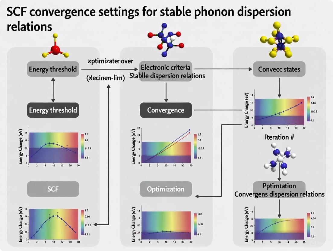
Achieving Stable Phonon Calculations: A Comprehensive Guide to SCF Convergence Settings
Calculating stable phonon dispersion relations is a critical but often challenging task in computational materials science, essential for predicting thermodynamic, mechanical, and transport properties.
Achieving Stable Phonon Calculations: A Comprehensive Guide to SCF Convergence Settings
Abstract
Calculating stable phonon dispersion relations is a critical but often challenging task in computational materials science, essential for predicting thermodynamic, mechanical, and transport properties. This article provides a comprehensive guide for researchers on establishing robust Self-Consistent Field (SCF) convergence protocols to ensure dynamical stability in phonon calculations. We cover the foundational relationship between electronic structure accuracy and lattice dynamics, detail methodological setups across different codes and material classes, present advanced troubleshooting for common instability issues, and outline best practices for validation against experimental data. By synthesizing insights from recent studies and high-throughput frameworks, this guide aims to equip scientists with the knowledge to reliably obtain physically meaningful phonon spectra, thereby accelerating the discovery of new functional materials.
The Critical Link Between Electronic Structure Accuracy and Phonon Stability
Why SCF Convergence is Non-Negotiable for Phonon Dispersion
In computational materials science, achieving a stable and accurate phonon dispersion relation is a fundamental goal for understanding lattice dynamics and thermodynamic properties. The integrity of this result is entirely dependent on the quality of the preceding self-consistent field (SCF) calculation. The SCF cycle is the iterative procedure that solves the Kohn-Sham equations in Density Functional Theory (DFT), where the Hamiltonian depends on the electron density, which in turn is obtained from the Hamiltonian [1]. Phonon calculations rely on second-order derivatives of the total energy with respect to atomic displacements, making them exceptionally sensitive to any inconsistencies or inaccuracies in the converged electronic structure. When SCF convergence is weak or incomplete, the resulting forces become unreliable, inevitably leading to unphysical imaginary frequencies in the phonon spectrum that distort the physical interpretation.
Essential SCF Convergence Criteria for Phonon Calculations
For reliable phonon dispersions, standard SCF tolerances are often insufficient. The convergence criteria must be tightened significantly to ensure the electronic structure is stable enough to produce accurate forces.
Table 1: Recommended SCF Convergence Criteria for Phonon Calculations
| Criterion | Standard Calculation | Phonon Calculation (Recommended) | Description |
|---|---|---|---|
| Energy Change (TolE) | 1e-6 Ha [2] | 1e-8 Ha or tighter [2] | Change in total energy between cycles |
| RMS Density Change (TolRMSP) | 1e-6 [2] | 5e-9 [2] | Root-mean-square change in density matrix |
| Maximum Density Change (TolMaxP) | 1e-5 [2] | 1e-7 [2] | Maximum element change in density matrix |
| DIIS Error (TolErr) | 1e-5 [2] | 5e-7 [2] | Error in the DIIS convergence accelerator |
| SCF Convergence Mode | Check change in energy [2] | Check all criteria (ConvCheckMode=0) [2] |
Ensures all aspects of the wavefunction are converged |
The ConvCheckMode is particularly crucial. While default settings might only check the energy change, phonon calculations require ConvCheckMode=0 in ORCA, which mandates that all convergence criteria are satisfied, providing a much more rigorous standard for wavefunction stability [2].
Advanced SCF Mixing Strategies for Difficult Systems
Metallic systems, magnetic materials, and structures with small band gaps often exhibit SCF convergence problems that can sabotage subsequent phonon calculations. Employing sophisticated mixing strategies is key to overcoming these issues.
Table 2: Comparison of SCF Mixing Algorithms
| Mixing Method | Mechanism | Best For | Key Parameters | Performance |
|---|---|---|---|---|
| Linear Mixing | Applies a simple damping factor to the new density/Hamiltonian [1] | Simple molecular systems, initial attempts | SCF.Mixer.Weight (Damping factor, e.g., 0.1-0.25) [1] [3] |
Robust but slow convergence; inefficient for difficult systems [1] |
| Pulay (DIIS) | Builds an optimized combination of past residuals to accelerate convergence [1] | Most systems (default in many codes) [1] [3] | SCF.Mixer.History (Number of past steps, default=2) [1] [3] |
Generally efficient and reliable [1] |
| Broyden | Quasi-Newton scheme updating mixing using approximate Jacobians [1] | Metallic systems, magnetic systems, non-collinear spin [1] | SCF.Mixer.History, SCF.Mixer.Weight [1] |
Similar to Pulay; can outperform in specific difficult cases [1] |
Most codes allow mixing either the Hamiltonian (SCF.Mix Hamiltonian) or the Density Matrix (SCF.Mix Density). For most modern calculations, mixing the Hamiltonian is the default and typically provides better results [1] [3].
The Scientist's Toolkit: Essential Computational Reagents
Table 3: Key "Research Reagent" Solutions for SCF and Phonon Calculations
| Reagent / Tool | Function | Role in Ensuring Stability |
|---|---|---|
| Tight SCF Convergence Settings | Stricter thresholds for energy, density, and gradient changes [2] | Foundation for accurate forces; prevents numerical noise in phonons |
| Pulay/DIIS Mixer | Advanced convergence accelerator using iteration history [1] | Solves charge sloshing in metals and oscillations in difficult spins |
| Electronic Smearing | Occupies orbitals with fractional electrons at finite temperature [4] | Smears degenerate states in metals/gaps; aids initial SCF convergence |
| Force Constant Supercell | Large enough real-space cell to capture atomic interactions [5] | Ensces phonon dynamical matrix includes all physically relevant interactions |
| Wigner-Seitz Scheme | Symmetry-conserving copying of periodic data in the supercell [5] | Preserves crystal symmetry in force constants; avoids imaginary frequencies |
Troubleshooting Guide: Resolving Imaginary Frequencies
FAQ 1: My phonon dispersion shows imaginary frequencies even after geometry optimization. What should I check first?
Answer: Imaginary frequencies indicate that the structure is not in a true minimum or that the force constants are inaccurate. Follow this systematic troubleshooting workflow:
First, verify that your SCF calculation is truly converged. Check the output to ensure it met all convergence criteria, not just the energy change. For phonons, using TightSCF or VeryTightSCF settings is non-negotiable [2]. Then, ensure your force constant calculation uses a sufficiently large supercell with proper symmetry handling (use_wigner_seitz_scheme=True in QuantumATK) [5]. Using a interaction cutoff shorter than the range of physical coupling will break crystal symmetry and likely produce imaginary frequencies [5].
FAQ 2: How can I improve SCF convergence for metallic systems before phonon calculations?
Answer: Metallic systems with vanishing band gaps are notoriously difficult for SCF convergence. Implement these specific protocols:
- Enable Electron Smearing: Apply a small electronic temperature (e.g., 0.01-0.001 Ha) to simulate fractional occupation of states near the Fermi level [6]. This helps overcome convergence issues in systems with many near-degenerate levels [4].
- Use Conservative DIIS Parameters: For extremely difficult cases, switch from aggressive to stable DIIS settings:
- Employ MultiSecant or LISTi Methods: As alternatives to DIIS, these methods can sometimes converge problematic systems more effectively [6].
- Adopt a Two-Stage Optimization: Use looser SCF criteria and smearing in initial geometry optimization steps, then tighten them as the geometry approaches its minimum [6].
FAQ 3: What specific SCF settings in ORCA ensure reliable phonons for transition metal complexes?
Answer: Open-shell transition metal complexes are challenging due to localized d-orbitals. Use these ORCA-specific settings:
The ConvCheckMode 0 flag is critical as it ensures all convergence criteria must be satisfied, not just one [2]. Additionally, for open-shell systems, always perform a stability analysis after SCF convergence to verify you have found a true minimum and not a saddle point on the orbital rotation surface [2].
FAQ 4: How do I troubleshoot "phonon dispersion doesn't match DOS" problems?
Answer: This discrepancy typically arises from different k-point and q-point sampling meshes. The DOS is derived from k-space integration over the entire Brillouin zone, while the dispersion plot follows a specific high-symmetry path [6].
Solution: Ensure your phonon DOS calculation uses a q-point mesh that is sufficiently dense to be converged. The --qpoint_grid 24 24 24 option (or similar in your code) should be tested for convergence [7]. Additionally, verify that the SCF calculation preceding the DOS uses a k-mesh of KSpace%Quality that is appropriate for the system [6].
Understanding the Impact of Numerical Parameters on the Dynamical Matrix
Frequently Asked Questions (FAQs)
1. How do SCF convergence criteria affect the accuracy of my phonon dispersion curves?
The Self-Consistent Field (SCF) convergence criteria directly impact the precision of the forces used to compute the force constants, which form the foundation of the dynamical matrix. Inaccurate SCF settings can lead to erroneous reporting of elastic properties and phonon frequencies. Setting the SCF convergence too loose may result in unphysical imaginary frequencies in your phonon dispersion, falsely indicating dynamical instability. For reliable results, studies often use stringent criteria, such as 10⁻⁵ Ry for total energy and 10⁻⁵ eV/Å for force minimization [8].
2. My phonon calculation shows imaginary frequencies. Is this always a sign of dynamical instability? Not necessarily. Imaginary frequencies (negative eigenvalues of the dynamical matrix) can be a genuine indicator of structural instability. However, they can also be numerical artifacts caused by insufficient parameters. Before concluding dynamical instability, you must verify that your calculation is numerically converged. Key parameters to check include the k-point grid density, energy cutoff, supercell size for the finite displacement method, and the SCF convergence criteria [9] [10]. For molecular crystals, the weak intermolecular interactions require particularly high numerical accuracy to avoid spurious imaginary modes [10].
3. What is the relationship between force constants and the dynamical matrix? The force constant matrix is the real-space representation of the interatomic force constants, calculated as the second derivative of the total energy with respect to atomic displacements. The dynamical matrix, (\mathbf{\Phi}(\mathbf{q})), is the Fourier transform of this mass-weighted force constant matrix [7]: [ \mathbf{\Phi}{ij}(\mathbf{q})= \sum{\mathbf{R}} \frac{ \mathbf{\Phi}{ij}(\mathbf{R}) }{\sqrt{mi m_j}} e^{i\mathbf{q}\cdot \mathbf{R}} ] where (i, j) are atom indices, (\mathbf{R}) is a lattice vector, (m) is atomic mass, and (\mathbf{q}) is the wave vector. The eigenvalues of the dynamical matrix give the squared phonon frequencies for each (\mathbf{q})-point [11].
4. Why is my phonon calculation so computationally expensive, and how can I make it more efficient? Phonon calculations are expensive because they require computing the force constant matrix. This involves performing multiple DFT calculations where each atom in a large supercell is displaced, leading to a number of calculations scaling with the number of atoms [12] [10]. For a system with (N) atoms in the supercell, you need (3N) displacement calculations. Efficiency can be improved by:
- Using space-group symmetries to reduce the number of unique displacements [12].
- For molecular crystals, employing the minimal molecular displacement (MMD) method, which uses rigid-body motions and key intramolecular modes, potentially reducing computational cost by a factor of 4 to 10 [10].
- Ensuring your supercell is large enough to capture all relevant interatomic interactions but not unnecessarily large [11].
Troubleshooting Guides
Problem: Non-Converged Phonon Frequencies
Symptoms:
- Phonon frequencies (especially low-energy ones) shift significantly when increasing the k-point density or energy cutoff.
- Appearance of small, spurious imaginary frequencies that change location or magnitude with numerical parameters.
Solution: Follow a systematic convergence procedure. The table below summarizes key parameters and their role.
Table: Key Numerical Parameters for Converged Phonon Calculations
| Parameter | Description | Convergence Strategy | Typical Effect of Non-Convergence |
|---|---|---|---|
| K-point Grid | Sampling density in the Brillouin zone. | Increase k-points until total energy changes are below a threshold (e.g., 10⁻⁴ Ry [8]). |
Inaccurate force constants, erroneous phonon frequencies and band gaps. |
| Energy Cutoff | Plane-wave basis set kinetic energy cutoff. | Increase cutoff until total energy converges. | Incomplete basis, inaccurate forces and lattice dynamics [9]. |
| SCF Criteria | Tolerance for electronic energy/force convergence. | Tighten until forces are stable (e.g., 10⁻⁵ eV/Å [8]). |
Noisy forces, inaccurate force constants, imaginary frequencies [9]. |
| Supercell Size | Size of the repeated cell for force constants. | Increase size until phonon frequencies at Brillouin zone boundary converge. | Aliasing: Incorrect description of long-wavelength phonons [11]. |
Experimental Protocol:
- Start with a Converged Ground State: Optimize your geometry until forces on atoms are minimal (e.g.,
< 0.01 eV/Å) [11] using a well-converged k-point grid and energy cutoff. - Converge the K-point Grid for the Supercell: The k-point grid for the force constant calculation should be commensurate with the supercell size. A common practice is to use a
Γ-centered1x1x1k-point mesh for the supercell, but this must be checked. - Select a Supercell: Choose a supercell large enough to capture the longest-range interatomic interactions relevant to your system. A common starting point is a
(5,5,5)or(7,7,7)supercell [12]. - Calculate Force Constants: Use the finite displacement method. The displacement value
deltamust be chosen carefully; a value that is too large introduces anharmonic effects, while one that is too small amplifies numerical noise. A typical value is0.01 Å[11]. - Check for Convergence: Repeat steps 2-4 with a larger supercell and/or denser k-point grid until the phonon frequencies of interest (e.g., at high-symmetry points) no longer change significantly.
Problem: Imaginary Frequencies in a Stable Material
Symptoms: The phonon dispersion curve shows imaginary (negative) frequencies, but experimental data or other theoretical evidence suggests the material should be dynamically stable.
Solution: This is often a numerical artifact. Follow this diagnostic flowchart to identify the root cause.
Diagram: Diagnostic flowchart for resolving imaginary frequency issues.
Verification Steps:
- Check Equilibrium Forces: Before displacing atoms, ensure the forces on all atoms in the optimized structure are close to zero. Large residual forces indicate an improperly relaxed structure, which will corrupt the force constants [12].
- Impose the Acoustic Sum Rule: The phonons must have three zero-frequency modes (acoustic modes) at the Brillouin zone center (Γ-point). Small numerical errors can break this condition. Most phonon codes include an option to impose the acoustic sum rule post-processing [12].
- Verify with a Different Method/Code: If possible, try an alternative method, such as Density Functional Perturbation Theory (DFPT), which calculates force constants in reciprocal space and can sometimes be more robust [13].
The Scientist's Toolkit
Table: Essential Research Reagents for Stable Phonon Calculations
| Reagent / Tool | Function / Purpose | Technical Notes |
|---|---|---|
| DFT Code (e.g., WIEN2k, GPAW) | Performs electronic structure calculations to obtain total energies and atomic forces. | Choose a code with demonstrated accuracy for your material class. Use the full-potential (FP) method for high precision [8]. |
| Phonon Software (e.g., ASE, TDEP) | Implements the finite displacement method, constructs the force constant and dynamical matrices, and calculates phonon dispersions/DOS. | Ensure the software can handle your crystal symmetry and implements corrections like the acoustic sum rule [12] [7]. |
| High-Performance Computing (HPC) Cluster | Provides the computational resources needed for the many DFT calculations involved in force constant computation. | A single phonon calculation for a medium-sized system can require hundreds to thousands of CPU hours [10]. |
| Stringent SCF Convergence Parameters | Ensures the electronic structure is fully converged at each step, leading to accurate and reliable forces. | Use criteria like 10⁻⁵ Ry for energy and 10⁻⁵ eV/Å for forces [8]. |
| Well-Converged K-point Grid | Ensures accurate sampling of the Brillouin zone for the electronic structure. | A dense grid (e.g., 1000 k-points in the irreducible wedge) is often necessary [8]. |
| Large Enough Supercell | Captures the real-space decay of interatomic force constants. | For molecular crystals, the supercell must be large enough to avoid interactions between periodic images of displaced molecules [10] [11]. |
Frequently Asked Questions
Q1: What is the fundamental link between the Kohn-Sham equations and lattice vibration calculations? The Kohn-Sham equations form the foundation of Density Functional Theory (DFT) by simplifying the many-electron problem into an auxiliary non-interacting system. This electronic structure solution provides the ground state energy and forces on atoms, which are essential inputs for calculating lattice vibrations (phonons). The harmonic approximation expands the crystal potential energy to second order in atomic displacements, with the force constants derived from these DFT-calculated forces. The dynamical matrix, whose eigenvalues give phonon frequencies, is built from these force constants [14] [15].
Q2: My SCF calculation fails to converge during phonon calculations. What strategies can I try? Slow or failed SCF convergence is common in systems with metallic character or complex electronic structures. Several proven strategies exist:
- SCF=QC: Use a quadratically convergent SCF procedure, which is slower but more reliable than default algorithms [16].
- Fermi broadening: Request temperature broadening during early iterations combined with CDIIS and damping for metallic systems [16].
- Damping: Enable dynamic damping of early SCF iterations, particularly when using CDIIS [16].
- Mixing parameters: Adjust
mixing_betaandmixing_modein Quantum ESPRESSO (mixing_beta = 0.7andmixing_mode = 'plain'are common starting points) [17]. - Tighter convergence: For phonon calculations, use higher energy cutoff values and tighter SCF convergence criteria (
conv_thr = 1.0e-8in Quantum ESPRESSO) for better accuracy [17].
Table 1: Essential SCF Convergence Options for Phonon Calculations
| Option | Function | Typical Use Case |
|---|---|---|
| SCF=QC | Quadratically convergent procedure [16] | Difficult convergence cases |
| SCF=Fermi | Temperature broadening [16] | Metallic systems |
| SCF=Damp | Dynamic damping [16] | Early SCF iterations |
| mixing_beta | Controls density mixing [17] | Most systems (0.7 default) |
| conv_thr | Convergence threshold [17] | Phonon calculations (1.0e-8) |
Q3: How do I handle imaginary frequencies (negative values) in my phonon dispersion? Imaginary frequencies (plotted as negative values) indicate dynamic instability where the crystal structure is not at a minimum in the potential energy surface [18]. First, verify technical factors: ensure supercell size convergence, use appropriate SCF convergence criteria, and check k-point sampling density. For polar materials, include LO-TO splitting corrections by calculating and providing Born effective charges and the dielectric tensor [15]. If instabilities persist after technical verification, they may be physical, indicating a structural phase transition or that the calculated structure is not the ground state [18].
Q4: What is LO-TO splitting and why is it crucial for polar materials? LO-TO splitting refers to the splitting of longitudinal optical (LO) and transverse optical (TO) phonon modes at the Brillouin zone center (Γ-point) in polar materials. This arises from long-range dipole-dipole interactions in materials with atoms carrying different Born effective charges [15]. Proper treatment requires:
- Computing Born effective charges and the static dielectric tensor using DFPT (
LEPSILON = .TRUE.in VASP) [15] - Providing these tensors as input to the phonon calculation (
LPHON_POLAR = .TRUE.,PHON_BORN_CHARGES, andPHON_DIELECTRICin VASP) [15] - Without this correction, phonon dispersions show unphysical behavior and inaccuracies near the Γ-point [15]
Q5: How do I choose between finite displacement and DFPT methods for phonons? The choice depends on your computational code, system, and requirements:
Table 2: Finite Displacement vs. DFPT for Phonon Calculations
| Aspect | Finite Displacement | Density Functional Perturbation Theory (DFPT) |
|---|---|---|
| Method | Numerical derivatives from atomic displacements [15] [19] | Analytical derivatives [15] [17] |
| Computational Cost | Many supercell calculations [19] | Typically fewer calculations [17] |
| Key Advantage | Broad applicability [20] | Efficiency for dense q-point sampling [20] |
| Limitation | Computationally expensive for large systems | Not available with all pseudopotentials/functionals [20] |
| Force Constants | From forces on displaced atoms [19] | Directly from 2nd-order derivative of energy [17] |
Q6: My phonon DOS looks jagged even with a reasonable q-point mesh. How can I fix this? A jagged density of states (DOS) indicates insufficient q-point sampling. Phonon DOS calculations require two levels of q-point convergence [21]:
- Coarse q-point grid: Explicitly calculate the dynamical matrix on a uniform mesh. Converge the DOS with respect to this grid size [21].
- Fine q-point grid: Interpolate the dynamical matrix onto a much denser mesh to obtain a smooth DOS. Fix the coarse grid and increase the fine mesh until the DOS profile converges [21].
For anisotropic cells, use a grid with uniform density in reciprocal space rather than equal points in all directions [21]. A common mistake is using only the coarse grid for the final DOS. The fine interpolation grid is essential for smooth curves.
Troubleshooting Guides
SCF Convergence Failure
Symptoms: Oscillating energy values, error messages about SCF convergence, or calculations exceeding maximum cycles.
Step-by-Step Resolution:
- Initial checks: Verify system charge and multiplicity settings. Use a well-converged charge density as the initial guess.
- Moderate interventions: Enable dynamic damping (
Dampin Gaussian [16],mixing_beta = 0.3in other codes) or Fermi broadening (SCF=Fermifor metals in Gaussian [16]). - Advanced strategies: Switch to quadratically convergent SCF (
SCF=QCin Gaussian [16]). Increase the SCF cycle limit (MaxCycle). - Last resorts: Gradually increase the planewave cutoff energy. For difficult metallic systems, use the
IALGO=48solver in VASP.
Imaginary Phonon Frequencies
Symptoms: Negative frequencies appearing in phonon dispersion or DOS, particularly at specific q-points.
Diagnosis and Resolution Workflow:
- Verify calculation parameters:
- Check for polar materials:
- Assess physical meaning: If technical issues are ruled out, imaginary frequencies may indicate genuine dynamic instability, suggesting a transition to a different crystal structure [18].
Inaccurate Phonon Frequencies in Polar Materials
Symptoms: Unphysical oscillations or discontinuities in phonon dispersion near Γ-point, incorrect LO-TO splitting.
Resolution:
- Calculate dielectric properties: Perform a DFPT calculation to obtain Born effective charges and the static dielectric tensor. In VASP, set
LEPSILON = .TRUE.[15]. Ensure this calculation is well-converged with respect to k-points and cutoff energy [15]. - Provide properties to phonon calculation:
- Verify results: Check that the LO-TO splitting is correctly reproduced by comparing with experimental data if available.
Experimental Protocols & Methodologies
Quantum ESPRESSO Phonon Dispersion Protocol
This protocol calculates phonon dispersion using DFPT in Quantum ESPRESSO [17]:
SCF Calculation (
pw.x):Run:
mpirun -np 4 pw.x -i pw.scf.in > pw.scf.outPhonon Calculation (
ph.x):Run:
mpirun -np 4 ph.x -i ph.in > ph.outq2r Transformation (
q2r.x):Run:
mpirun -np 4 q2r.x -i q2r.in > q2r.outDispersion Calculation (
matdyn.x):Run:
mpirun -np 4 matdyn.x -i matdyn.in > matdyn.out
VASP Finite Displacement Protocol (via phonopy)
This protocol uses the finite displacement method with VASP and phonopy [19]:
Pre-process (generate displaced supercells):
Generates
SPOSCARandPOSCAR-001,POSCAR-002, etc.VASP Force Calculations (for each
POSCAR-{number}): Use thisINCARtemplate:Ensure
NSW = 0orIBRION = -1to prevent structural relaxation.Create Force Constants:
Creates
FORCE_SETSfile.Post-process (plot DOS and bands):
Dielectric Property Calculation for Polar Materials
This standalone VASP calculation obtains Born effective charges and dielectric tensor needed for LO-TO splitting corrections [15]:
INCAR Settings:
Execution:
Extracting Results:
- Born effective charges and dielectric tensor are written to
OUTCAR,vasprun.xml, andvaspout.h5[15]. - For phonopy, create the
BORNfile using:phonopy-vasp-born[19].
Workflow Visualization
Phonon Calculation Workflow from Kohn-Sham Equations to Phonon Properties
The Scientist's Toolkit: Research Reagent Solutions
Table 3: Essential Computational Tools for Phonon Calculations
| Tool/Component | Function | Implementation Examples |
|---|---|---|
| SCF Convergence Algorithms | Solve Kohn-Sham equations iteratively [16] | DIIS, CDIIS, Fermi broadening, Quadratically Convergent (QC) [16] |
| Pseudopotentials | Represent core electrons, reduce computational cost [17] | Norm-conserving (NCP), Ultrasoft (USP), PAW datasets [20] |
| Phonon Methods | Calculate force constants/dynamical matrix [20] | Finite Displacement (supercell), Density Functional Perturbation Theory (DFPT) [15] [20] |
| Symmetry Analysis | Reduce computational cost, classify modes [20] | Space group analysis, Irreducible representations, Point group character tables [20] |
| Dielectric Properties | Handle long-range interactions in polar materials [15] | Born effective charges, Static dielectric tensor [15] |
| Post-Processing Tools | Analyze and visualize phonon properties [19] | phonopy, CRYSPLOT, matdyn.x, phonopy-load [22] [17] [19] |
| Sum Rule Corrections | Impose physical constraints on calculations [20] | Acoustic sum rule (ASR) enforcement [20] |
Frequently Asked Questions
What is the physical meaning of an imaginary frequency? An imaginary frequency, mathematically represented as a complex number where the real part is zero and the imaginary part is non-zero, indicates an exponential decay or growth of a vibrational mode over time rather than a stable oscillation [23] [24]. In the context of phonon calculations, it signals a dynamical instability in the crystal structure or molecular geometry [24].
Are imaginary frequencies always a sign of a problem? In the context of locating equilibrium geometries, yes. They indicate that the current structure is not a local minimum on the potential energy surface but rather a transition state or saddle point. However, they are physically meaningful in other contexts, such as representing damping phenomena or, in theoretical physics, Matsubara frequencies in statistical mechanics [24].
What is the difference between a real and an imaginary frequency? A real frequency corresponds to a stable, oscillatory motion of atoms around their equilibrium positions. An imaginary frequency describes a mode where atomic displacements lead to a decrease in energy, causing the structure to move towards a different, more stable configuration.
Imaginary frequencies often result from inaccuracies in the underlying calculations. The following workflow outlines a systematic approach to diagnose and resolve their most common sources.
Source 1: Poor Self-Consistent Field (SCF) Convergence
An unconverged SCF calculation produces an inaccurate electron density, which leads to erroneous forces and, consequently, unphysical force constants [25].
- Diagnosis: Check the SCF output for oscillations in the energy or orbital occupations. The calculation may report "SCF not fully converged!" [26] [25].
- Solution Protocol:
- Increase iterations: Increase the maximum number of SCF cycles (
MaxIter 500) [26]. - Use advanced convergers: Employ more robust algorithms like the Trust Radius Augmented Hessian (TRAH) or KDIIS [26].
- Improve initial guess: Use
MOReadto import orbitals from a simpler, converged calculation (e.g., BP86/def2-SVP) [26]. - Apply damping: For difficult systems (e.g., open-shell transition metals), use the
SlowConvorVerySlowConvkeywords to dampen oscillations [26].
- Increase iterations: Increase the maximum number of SCF cycles (
Source 2: Incorrect or Unphysical Geometry
The calculation may be performed on a molecular geometry that is not a true energy minimum, such as a structure with strained bonds or atoms too close together [25].
- Diagnosis: Visually inspect the atomic structure. Check for unrealistically long or short chemical bonds, or implausible angles.
- Solution Protocol:
- Re-optimize geometry: Perform a careful geometry optimization, possibly using a different functional or basis set initially.
- Verify coordinates: Ensure the input geometry uses the correct units (e.g., angstroms vs. bohrs) and is chemically sensible [25].
Source 3: Inadequate Treatment of Force Constants
In phonon calculations, the dynamical matrix is built from force constants. If the supercell used to compute them is too small, or the long-range interactions in polar materials are not handled correctly, it can introduce instabilities [7] [15].
- Diagnosis: Imaginary frequencies, especially at the Γ-point or leading to unphysical "overshooting" in the dispersion curves [15].
- Solution Protocol:
Source 4: Artificially High Symmetry
Imposing symmetry that is incompatible with the true electronic ground state can force degenerate orbitals, resulting in a vanishing HOMO-LUMO gap and SCF convergence issues that manifest as imaginary frequencies [25].
- Diagnosis: Imaginary frequencies appear when using high symmetry, but disappear in a lower-symmetry calculation.
- Solution Protocol:
- Lower symmetry: Relax the geometry without symmetry constraints (
Nosymor similar keyword). - Check electronic state: Ensure the calculation is configured for the correct spin state, especially for transition metal complexes [25].
- Lower symmetry: Relax the geometry without symmetry constraints (
The Scientist's Toolkit: Research Reagent Solutions
The following table details key computational tools and parameters essential for stable phonon calculations.
| Item/Reagent | Function | Protocol & Specification |
|---|---|---|
| SCF Convergers | Algorithms to find a self-consistent electron density field. | TRAH: Robust but expensive; use for difficult cases [26]. KDIIS+SOSCF: Faster convergence for standard systems [26]. |
| Force Constants | Matrix elements describing harmonic interactions between atoms. | Supercell Size: Must be converged; use IBRION=5,6,7,8 in VASP [15]. Long-range Corrections: Essential for polar materials [15]. |
| Born Effective Charges & Dielectric Tensor | Materials properties quantifying long-range dipole-dipole interactions. | Calculation: Obtain from a DFPT calculation (LEPSILON or LCALCEPS). Input: Specify via PHON_BORN_CHARGES and PHON_DIELECTRIC [15]. |
| Q-point Path & Mesh | Set of points in reciprocal space for sampling phonons. | Dispersion: Use a high-symmetry path (e.g., 100 points between high-symmetry points) [7]. DOS: Use a dense, uniform mesh (e.g., 24x24x24) [7]. |
Experimental Protocol for Stable Phonon Dispersion
This protocol outlines the key steps for obtaining reliable, instability-free phonon dispersion relations, integrating the troubleshooting concepts above.
Step 1: Robust Unit Cell Optimization
- Action: Optimize the geometry of the primitive cell with high-precision SCF settings.
- Methodology: Use a functional and basis set appropriate for the system. Employ
Tightoptimization criteria and confirm the absence of imaginary frequencies in the resulting Hessian. This ensures you start from a true local minimum [25].
Step 2: Accurate Force Constant Calculation
- Action: Compute the interatomic force constants in a sufficiently large supercell.
- Methodology: Use density-functional perturbation theory (
IBRION=7,8in VASP) or the finite-displacement method. The supercell size must be converged so that the force constants for atoms at the boundary are negligible [15].
Step 3: Phonon Property Calculation
- Action: Construct the dynamical matrix and diagonalize it across the Brillouin zone.
- Methodology: Fourier interpolate the force constants onto a path of q-points for the dispersion relation and a dense mesh of q-points for the phonon Density of States (DOS). For polar materials, the Born effective charges and dielectric tensor must be included to handle the non-analytical part of the dynamical matrix at the Γ-point [7] [15].
Step 4: Analysis and Validation
- Action: Interpret the results and validate the calculation.
- Methodology: Examine the phonon dispersion for any imaginary frequencies (plotted as negative values). If present, follow the troubleshooting guide. Validate the results against experimental data like Raman or IR spectra, if available.
Practical Protocols: Implementing Robust SCF Settings Across Different Systems
This guide provides a detailed workflow and troubleshooting advice for obtaining stable phonon dispersion relations, with a specific focus on the critical role of Self-Consistent Field (SCF) convergence settings.
Complete Workflow Diagram
The following diagram outlines the core steps for moving from an initial structure to a successful phonon calculation, highlighting key decision points and convergence checks.
Frequently Asked Questions
What are the most critical SCF parameters for a stable geometry optimization preceding phonon calculations?
Tight control of SCF convergence is essential for generating reliable geometries for subsequent phonon analysis. Inaccurate forces due to poor SCF convergence propagate through geometry optimization and negatively impact phonon stability.
SCF Convergence Parameter Table
| Parameter | Recommended Value | Purpose |
|---|---|---|
Convergence%Criterion |
1e-6 to 1e-8 (or tighter) [27] |
Primary density convergence threshold |
SCF%Iterations |
300+ [27] | Maximum SCF cycles allowed |
SCF%Method |
MultiSecant or DIIS [27] [6] |
Algorithm for density convergence |
SCF%Mixing |
0.05-0.075 [27] [6] | Damping parameter for potential update |
Convergence%ElectronicTemperature |
0.0 (final value) [27] | Smearing for initial convergence |
For difficult systems, implement adaptive SCF settings during geometry optimization using EngineAutomations to gradually tighten convergence criteria as the geometry approaches its minimum [6].
How do I troubleshoot SCF convergence failures during geometry optimization?
SCF convergence problems often manifest as oscillating energies or failure to meet convergence criteria within the maximum cycle limit.
SCF Convergence Troubleshooting Table
| Problem | Solution | Rationale |
|---|---|---|
| SCF oscillates | Decrease SCF%Mixing to 0.05 [6] |
Reduces step size in potential updates |
| DIIS instability | Use SCF%Method MultiSecant [6] |
Alternative algorithm with better stability |
| Slow convergence | Enable Convergence%Degenerate Default [27] [6] |
Smears occupations near Fermi level |
| Small HOMO-LUMO gap | Apply energy level shifting (if available) [28] | Increases virtual-occupied orbital gap |
| Poor initial guess | Use InitialDensity psi [27] or start from atomic orbitals |
Provides better starting density |
Additional advanced options include using the LISTi method (DIIS%Variant LISTi) [6] or improving numerical accuracy through NumericalQuality Good [6].
Why does my phonon calculation show negative frequencies, and how can I fix it?
Negative (imaginary) frequencies in phonon spectra indicate dynamical instability, where the crystal structure is not at a true minimum.
Solutions for Negative Frequencies
Improve Geometry Optimization Quality
- Tighter Force Convergence: Ensure nuclear gradients are sufficiently small [6]
- Optimize Lattice Vectors: For solid-state systems, enable lattice optimization with "Very Good" convergence thresholds [29]
- Tighter SCF Convergence: Use stricter criteria (
1e-7to1e-8) during the final optimization steps [9]
Enhance Computational Parameters
Electronic Structure Considerations
How should I converge q-points for phonon density of states calculations?
Accurate phonon density of states requires proper convergence with respect to q-point sampling.
Two-Grid Convergence Strategy
- Coarse Grid Convergence: Systematically increase the grid of explicitly calculated q-points until the DOS profile stabilizes [21]
- Fine Interpolation Grid: Use Fourier interpolation on a much denser grid than the converged coarse grid for smooth DOS [21]
Practical Implementation
- Begin with a fixed, dense fine grid (e.g., 30×30×30)
- Increase coarse grid size until DOS converges
- Use uniform density grids, adjusting point counts inversely with lattice constants [21]
- For DFPT calculations, these are the q-points where response is explicitly calculated [21]
What are the essential research reagent solutions for phonon calculations?
Computational Materials Toolkit
| Item | Function | Application Notes |
|---|---|---|
| DFTB Parameters | Preparameterized Hamiltonians | Use established sets (e.g., DFTB.org/hyb-0-2) [29] |
| Pseudopotentials | Electron-ion interactions | Ensure consistent accuracy with functional |
| Basis Sets | Electronic wavefunction expansion | Apply confinement to avoid linear dependency [6] |
| Phonon Software | Lattice dynamics calculation | PHONOPY, ShengBTE, or built-in modules [30] |
| Visualization Tools | Results analysis | AMSbandstructure, VESTA, XCrySDen [29] |
Key Technical Recommendations
For reliable phonon calculations, ensure proper workflow sequencing: (1) achieve high-quality geometry optimization with tight SCF and force convergence, (2) verify the absence of imaginary frequencies, and (3) perform q-point convergence tests for DOS calculations. The most common cause of unstable phonons is insufficient geometry optimization quality, often remedied by tighter SCF convergence criteria and lattice parameter optimization [29] [6] [31].
Technical Support Center
Troubleshooting Guide: SCF Convergence for Stable Phonon Calculations
This guide addresses common challenges in achieving self-consistent field (SCF) convergence, a critical prerequisite for obtaining stable and physically meaningful phonon dispersion relations in ab initio simulations.
FAQ 1: How do I resolve persistent SCF oscillations in my phonon calculations?
Issue: The total energy oscillates between values without converging.
Diagnosis: This often stems from an inappropriate charge mixing scheme or parameters.
Resolution:
- Reduce
mixing_beta: Lower the mixing parameter (e.g., from 0.7 to 0.3 or 0.2) to reduce the amount of new charge density mixed in each step [32]. - Increase
mixing_ndim: Increase the number of previous steps used in the mixing (e.g., from 8 to 16). This helps dampen oscillations by providing a broader history for the mixing algorithm [32]. - Change
mixing_mode: Switch to a more robust mixing algorithm, such as `local-TF' (local Thomas-Fermi) for systems with strong charge inhomogeneities [32]. - Use
startingpot: Start from a superposition of atomic potentials if you suspect the initial potential is far from the solution [32].
Experimental Protocol:
- Begin with a default
mixing_betaof 0.7. - If oscillations occur, reduce
mixing_betain steps of 0.1. - If oscillations persist, double the
mixing_ndimparameter. - For complex metallic systems, consider using the Broyden mixing scheme if available.
FAQ 2: My phonon dispersion shows imaginary frequencies (instabilities). Are they physical or due to poor convergence?
Issue: The calculated phonon frequencies at some wavevectors are imaginary, indicating a dynamical instability.
Diagnosis: This can be due to a genuine structural instability or numerical inaccuracies from insufficient SCF convergence, k-point sampling, or energy cutoffs [33] [34].
Resolution:
- Verify SCF Convergence: Ensure the SCF energy convergence threshold (
conv_thr) is tight enough (typically1.0e-8Ry or lower for phonons). Forces used to compute interatomic force constants (IFCs) are highly sensitive to the electron density accuracy [32]. - Check k-point Grid Convergence: Perform a convergence test for the total energy and forces with respect to k-point grid density. An under-converged k-grid can lead to inaccurate forces and spurious instabilities.
- Confirm Energy Cutoff Convergence: Ensure the plane-wave kinetic energy cutoff (
ecutwfc) and charge density cutoff (ecutrho) are sufficiently high. Use a consistent cutoff value across all displacement calculations for IFCs. - Investigate Anharmonicity: If convergence parameters are adequate, the instabilities may be physical. For strongly anharmonic systems, standard harmonic calculations may fail, and advanced methods like the self-consistent harmonic approximation (SCHA) or temperature-dependent effective potential (TDEP) may be required [33].
Experimental Protocol for k-point Convergence:
- Select a representative structure (e.g., the equilibrium primitive cell).
- Calculate the total energy for a series of increasingly dense k-point grids (e.g., 2x2x2, 4x4x4, 6x6x6).
- Plot the total energy versus the inverse of the k-point grid density. The converged value is where the energy change is less than the desired
conv_thr. - Use this converged k-point grid for all subsequent electronic and phonon calculations.
Essential Parameters and Materials for Phonon Research
Key Parameter Tables for SCF Convergence
Table 1: Common SCF Convergence Parameters in Quantum ESPRESSO's ELECTRONS namelist [32].
| Parameter | Description | Typical Values | Function |
|---|---|---|---|
electron_maxstep |
Maximum SCF iterations | 100 - 200 | Prevents infinite loops in difficult convergence cases. |
conv_thr |
SCF convergence threshold | 1.0e-8 to 1.0e-10 Ry | Target accuracy for total energy; crucial for force accuracy in phonons. |
mixing_beta |
Mixing parameter for charge | 0.3 - 0.7 | Controls stability; lower values can dampen oscillations. |
mixing_mode |
Charge mixing algorithm | 'plain', 'TF', 'local-TF' | Algorithm used for mixing charge/potential from previous steps. |
mixing_ndim |
Number of iterations used in mixing | 4 - 16 | Higher values can improve stability of convergence. |
diagonalization |
Algorithm for band energy minimization | 'david', 'cg' | 'cg' (Conjugate Gradient) can be more stable than 'david' (Davidson). |
Table 2: Key Parameters for k-points and Energy Cutoffs in Quantum ESPRESSO's SYSTEM namelist [32].
| Parameter / Card | Description | Function |
|---|---|---|
ecutwfc |
Plane-wave kinetic energy cutoff | Determines the basis set size for wavefunctions. Must be converged. |
ecutrho |
Charge density cutoff | Typically 4x or 8x ecutwfc. Critical for ultrasoft pseudopotentials. |
K_POINTS |
k-points sampling scheme | 'automatic' for MP grids or explicit lists. Density is system-dependent. |
Research Reagent Solutions: Computational Tools for Phonon Studies
Table 3: Essential Software Tools for Ab Initio Phonon Calculations.
| Tool / "Reagent" | Function / Role | Application in Workflow |
|---|---|---|
| Quantum ESPRESSO (pw.x) [32] | DFT Main Engine | Performs the core electronic structure calculation to obtain total energies and forces. |
| DFPT Codes [20] | Linear Response Solver | Efficiently calculates second-order IFCs and phonon frequencies directly in reciprocal space. |
| Phonopy / Phono3py [33] | Post-Processing & Analysis | Extracts harmonic and anharmonic IFCs from force-displacement data via finite-difference method. |
| Pheasy [33] | Advanced IFC Extraction | Uses machine learning to efficiently extract high-order anharmonic IFCs from force-displacement datasets. |
| CASTEP [20] | Integrated DFT & Phonon Code | Provides both finite-displacement and DFPT methods for phonons within a single package. |
Workflow and Relationship Diagrams
Diagram: SCF Convergence Troubleshooting Pathway
Diagram: Interrelationship of Parameters for Stable Phonons
The pursuit of stable phonon dispersion relations is a cornerstone of computational materials science, directly impacting the prediction of thermodynamic properties, mechanical stability, and transport phenomena. Achieving self-consistent field (SCF) convergence is not merely a procedural step but a fundamental prerequisite for reliable phonon calculations. The electronic structure configuration found by the SCF method forms the basis for evaluating interatomic forces and, consequently, the dynamical matrix. Convergence problems frequently occur in systems with small HOMO-LUMO gaps, localized open-shell configurations (common in d- and f-elements), and transition state structures with dissociating bonds. Non-physical calculation setups, including high-energy geometries, also contribute to these challenges. This technical guide provides material-specific protocols and troubleshooting methodologies to overcome these obstacles, ensuring robust phonon calculations across different material classes.
Material-Specific Calculation Methodologies
Phonon Methods and Their Applicability
The choice of phonon calculation method is critical and depends on the material system, Hamiltonian, and desired properties. The following table summarizes the implementation restrictions and recommended approaches based on the CASTEP framework [20].
Table 1: Phonon Method Implementation Matrix and Recommendations
| Method / Hamiltonian | DFPT (Phonon) | DFPT (E-field) | FD (Phonon) | Recommended for Properties |
|---|---|---|---|---|
| Norm-Conserving Pseudopotentials (NCP) | ✓ | ✓ | ✓ | All properties |
| Ultrasoft Pseudopotentials (USP) | ✘ | ✘ | ✓ | IR/Raman with Berry Phase (Z^{*}) |
| LDA, GGA | ✓ | ✓ | ✓ | All properties with DFPT |
| DFT+U | ✘ | ✘ | ✓ | Phonon dispersion/DOS with FD |
| DFT+D: D3, D4 | ✘ | ✓ | ✓ | IR intensities with E-field; FD for phonons |
| PBE0, Hybrid XC | ✘ | ✘ | ✓ | Phonon dispersion/DOS with FD |
| Target Property | Preferred Method | |||
| IR/Raman Spectra | DFPT at q=0 (NCP) or FD at q=0 (USP) | |||
| Born Charges ((Z^{*})) | DFPT E-field (NCP) or Berry Phase (USP) | |||
| Phonon Dispersion/DOS | DFPT + Interpolation (NCP) or FD (USP/NCP) | |||
| Vibrational Thermodynamics | Same method as for DOS |
Metals and Semiconductors
Metals and small-unit-cell semiconductors are often well-described by semilocal DFT and are suitable for efficient Density-Functional Perturbation Theory (DFPT).
Example Protocol: DFPT at Γ-point for Semiconductors (e.g., Boron Nitride) [20]
The input file (seedname.cell) requires specific keywords to initiate a phonon calculation. Key components include:
- Cell and Positions: Defined using
LATTICE_ABCandPOSITIONS_FRACblocks. - Pseudopotentials: Specified in the
SPECIES_POTblock. - k-points: Set using
kpoints_mp_spacing. - Phonon Task: The
task : PHONONkeyword is essential. - Phonon Wavevector: The
PHONON_KPOINT_LISTblock specifies the wavevector(s) for the phonon calculation, typically starting with (0,0,0) for Γ-point properties.
SCF Convergence Guidance [4] For difficult-to-converge metallic systems with small gaps, the following strategies are recommended:
- Electron Smearing: Introduces fractional occupation numbers to distribute electrons over near-degenerate levels. Use a small smearing parameter and consider multiple restarts with successively smaller values.
- SCF Accelerators: For systems with strong fluctuations in SCF error, switch from the default DIIS to more stable algorithms like MESA or LISTi.
- DIIS Tuning: For a slower but more stable convergence, manually adjust DIIS parameters:
Molecular Crystals
Molecular crystals present a unique challenge due to large unit cells and weak intermolecular interactions (e.g., van der Waals forces), which require high numerical accuracy. The frozen-phonon (finite displacement) method is typically the preferred technique [35].
Novel Protocol: Minimal Molecular Displacement (MMD) Method [35] This method reduces the computational cost of frozen-phonon calculations in molecular crystals by up to a factor of 10 by using a basis of molecular displacements instead of individual atomic displacements.
Workflow Overview:
- Isolated Molecule Calculation: Compute the intramolecular normal modes for an isolated molecule.
- Crystal Supercell Calculation: Perform a single-point calculation for the full crystal to capture the electronic structure in the periodic environment.
- Force Constant Calculation: The dynamical matrix is built by combining the intramolecular force constants from step 1 with intermolecular force constants obtained from a limited number of supercell calculations where rigid molecular units are displaced.
- Phonon Spectrum Construction: The complete phonon spectrum, including the challenging and dispersive low-frequency region, is constructed from the force constant matrix.
This approach is particularly effective for the low-frequency lattice vibrations (below 200 cm⁻¹) which are crucial for thermodynamics and charge transport in organic semiconductors.
Standard Protocol: Finite Displacement with Quantum ESPRESSO [36] A common workflow for obtaining phonons and related properties using the finite displacement method involves:
- SCF Calculation: A self-consistent calculation on the primitive cell.
- Phonon Calculation: Run
ph.xwithldisp = .true.on a homogeneous q-grid (e.g., 4x4x4) to generate dynamical matrix files (si.dynX). - Force Constants: Use
q2r.xto compute the interatomic force constants (IFCs) from the dynamical matrices. - Phonon Dispersion: Use
matdyn.xto compute the phonon frequencies along a path in the Brillouin zone, generating a file that can be plotted.
FAQs and Troubleshooting Guides
SCF Convergence Failure
Q: My SCF calculation oscillates or diverges, especially during a geometry optimization. What are the first steps I should take?
A: Follow this systematic troubleshooting guide [4]:
- Verify Physical System: Ensure bond lengths and angles are realistic. Confirm the correct units (e.g., Ångstroms) were used for atomic coordinates.
- Check Spin Multiplicity: Use spin-unrestricted calculations for open-shell systems and manually set the correct spin components.
- Initial Electronic Guess: For a single-point calculation, try restarting from a moderately converged electronic structure from a previous calculation. In geometry optimization, the initial steps may be slow, but subsequent steps often converge more easily as the electronic structure is reused.
- Adjust SCF Algorithm:
- Change the convergence accelerator to a more stable method like MESA or LISTi.
- If using DIIS, increase the number of expansion vectors (
N 25) and the number of initial equilibration cycles (Cyc 30), while significantly reducing the mixing parameter (Mixing 0.015).
Handling Negative Frequencies
Q: I have obtained negative (imaginary) frequencies in my phonon dispersion. Does this always indicate a structural instability?
A: Not necessarily. While true imaginary frequencies can indicate a structural instability, they can also arise from numerical issues. Investigate the following:
- Supercell Size: Ensure the supercell used for the finite displacement calculation is large enough to capture long-range interactions, especially in ionic materials.
- SCF Convergence: Tighten the SCF convergence threshold in the force calculations (
tr2_phin Quantum ESPRESSO) to ensure forces are well-converged [36]. - k-point Sampling: Use a denser k-point grid for the initial electronic structure calculation.
- Symmetry: Apply acoustic sum rules (e.g.,
phonon_sum_rule : TRUEin CASTEP,asr='simple'in Quantum ESPRESSO) to enforce physical conditions on the dynamical matrix [20] [36]. - Physical vs. Numerical: If the imaginary frequencies are small (< 10-20 cm⁻¹) and isolated, they are likely numerical artifacts. If they are large and form a pattern, they may point to a genuine instability.
Method Selection for Specific Properties
Q: Which phonon method should I use to calculate Raman spectra for a system using ultrasoft pseudopotentials and DFT+U?
A: As shown in Table 1, DFPT is not implemented for ultrasoft pseudopotentials or DFT+U in some codes [20]. You must use the finite displacement (frozen-phonon) method. To obtain Raman intensities, you will need to couple the finite displacement calculation with a subsequent Berry phase evaluation of the dielectric susceptibility, as DFPT-based Raman is not available for your Hamiltonian setup.
The Scientist's Toolkit: Essential Computational Materials
Table 2: Key Software and Computational Tools for Phonon Calculations
| Tool / Reagent | Function / Purpose | Example Use Case |
|---|---|---|
| CASTEP | A DFT code using a plane-wave basis set for periodic systems. | DFPT calculation of IR and Raman spectra at the Γ-point for semiconductors [20]. |
| Quantum ESPRESSO (pw.x, ph.x) | An integrated suite of Open-Source DFT codes for electronic-structure calculations. | Finite displacement phonon calculations and generation of interatomic force constants [36]. |
| EPW (ZG.x) | An code for electron-phonon coupling and temperature-dependent properties. | Generating special displacement configurations for anharmonic and temperature-dependent band structure calculations [36]. |
| Norm-Conserving Pseudopotentials (NCP) | Pseudopotentials that preserve the charge density outside the core region. | Required for DFPT calculations of IR and Raman intensities in CASTEP [20]. |
| Ultrasoft Pseudopotentials (USP) | Pseudopotentials that allow for a lower plane-wave cutoff energy. | Used in finite-displacement phonon calculations when high efficiency is needed [20]. |
| Interatomic Force Constants (IFCs) | The second-order derivatives of the total energy with respect to atomic displacements. | The central quantity computed by ph.x & q2r.x; used for phonon dispersion and DOS [36]. |
Workflow Visualization
The following diagram illustrates the high-level decision process for selecting and executing a phonon calculation, integrating the material-specific considerations and methods discussed.
Diagram 1: Decision workflow for phonon calculations, highlighting method selection based on material and Hamiltonian.
Leveraging Automated Workflow Tools (e.g., atomate2) for High-Throughput Screening
Troubleshooting Guides
MongoDB Connection Issues
Problem: atomate2 workflows fail to connect to the MongoDB database, which is essential for storing calculation outputs and job states [37].
Diagnosis and Solution:
- Check Firewall Settings: Many high-performance computing (HPC) centers have firewalls that block database connections. Verify your center's policy. Solutions include contacting your computing center to allow connections, hosting the database within the supercomputing network, or using a proxy service [37].
- Verify Credentials: Ensure the
jobflow.yamlconfiguration file uses absolute paths and correct credentials. The file should be located in a secure, user-accessible directory [37]. - MongoDB Atlas Configuration: If using MongoDB Atlas, ensure the connection string in
jobflow.yamluses theMongoURIStoreandGridFSURIStoretypes. Add your cluster's IP address to the Atlas whitelist and create a dedicated database user [37].
SCF Convergence Failures in VASP Calculations
Problem: The Self-Consistent Field (SCF) procedure in electronic structure calculations (e.g., VASP) fails to converge, halting workflows. This is common in systems with transition metals, open-shell configurations, or small HOMO-LUMO gaps [26] [4].
Diagnosis and Solution:
- Increase SCF Iterations: For calculations that almost converge, increase the maximum number of SCF cycles [26].
- Use Advanced SCF Algorithms: For difficult cases (e.g., open-shell transition metal complexes), employ more robust but expensive algorithms. In ORCA, the Trust Radius Augmented Hessian (TRAH) method is designed for such systems [26].
- Employ Damping and Level Shifting: For oscillating or slowly converging SCF, use damping (e.g.,
ALGO = Allin VASP) or level shifting to stabilize convergence [26] [4]. - Improve Initial Guess: Converge a calculation with a simpler functional (e.g., BP86) or a closed-shell state, and use its orbitals as the initial guess for the target calculation [26].
Incorrect Phonon Dispersion Curves
Problem: Calculated phonon dispersion relations show imaginary frequencies (negative values on the plot), indicating structural instability or errors in the calculation setup [38].
Diagnosis and Solution:
- Verify Ground-State Structure: Phonon calculations require a fully optimized, equilibrium geometry. Ensure your initial structural optimization is complete and converged to tight tolerances [38].
- Check Supercell Convergence: Phonon calculations using the finite displacement method require a sufficiently large supercell to capture all atomic interactions. Systematically increase the supercell size until the phonon frequencies converge [38].
- Ensure Accurate Force Calculations: The force constants are derived from the forces induced by atomic displacements. Use high-precision electronic structure settings (e.g.,
PREC = Accuratein VASP, tighter SCF convergence) to ensure force accuracy [38].
Frequently Asked Questions (FAQs)
Q1: What are the software and environment prerequisites for running atomate2?
Atomate2 requires Python 3.10+. We recommend installing it within a Conda environment. Core dependencies include pymatgen for structure analysis, custodian for job management and error handling, and jobflow for workflow design. An optional dependency like jobflow-remote or FireWorks is needed for executing workflows on HPC systems [37].
Q2: My VASP calculation converges slowly for a metallic system. What SCF settings should I adjust?
For metals, enabling electron smearing (e.g., ISMEAR = 1 or 2 in VASP) is crucial. This assigns fractional occupancies to orbitals near the Fermi level, which stabilizes the SCF convergence. Keep the smearing parameter (SIGMA) as low as possible to minimize its effect on the total energy [4].
Q3: What is the difference between acoustic and optical phonon branches, and why does it matter?
- Acoustic Phonons: Represent in-phase atomic motions, dominate at low frequencies, and have a linear dispersion near the Brillouin zone center (Γ-point). Their slope determines the speed of sound in the material [38] [39].
- Optical Phonons: Represent out-of-phase atomic motions, typically exist at higher frequencies, and have flatter dispersion curves. They are important for properties like infrared absorption and Raman scattering [38] [39]. Understanding this distinction is vital for interpreting phonon dispersion plots and relating them to a material's thermal and vibrational properties [38] [39].
Q4: Can I use atomate2 for non-VASP codes?
While the initial implementation of atomate2 is heavily VASP-centric, its modular design, built on the jobflow library, allows for the creation of workflows for other simulation codes. The core concepts of workflows, makers, and job stores are code-agnostic [40].
Experimental Protocols & Workflows
Standard Workflow for Phonon Dispersion Calculation
This protocol outlines the steps to calculate phonon dispersions using atomate2 and VASP.
1. Structure Optimization
- Objective: Relax the atomic positions and cell vectors to find the ground-state equilibrium structure.
- Method: Use the
RelaxBandStructureMakeror a dedicatedRelaxMakerin atomate2. - Key Parameters:
- Functional: e.g., PBE.
- Pseudopotential: e.g., PAW-PBE.
- k-point density: > 50 /Å⁻³.
- Force convergence: < 0.01 eV/Å.
2. Self-Consistent Static Calculation on Relaxed Geometry
- Objective: Obtain a high-accuracy charge density on a dense k-point mesh.
- Method: A static calculation (
StaticMaker) using the optimized structure. - Key Parameters:
- k-point density: Higher than the optimization step.
- SCF convergence:
TightorVeryTightsettings.
3. Non-Self-Consistent Field (NSCF) Calculations
- Objective: Calculate the electronic density of states (DOS) and band structure.
- Method: Two separate NSCF runs are typically performed:
- Uniform Mesh: For DOS.
- High-Symmetry Path: For the electronic band structure.
4. Phonon Calculation via Finite Displacement
- Objective: Calculate the interatomic force constants.
- Method: Use a
PhononMakerworkflow. This involves creating a supercell and performing multiple single-point calculations where each atom is displaced slightly from its equilibrium position. The forces from these calculations are used to construct the dynamical matrix. - Key Parameters:
- Supercell size: Must be large enough to capture long-range interactions.
- Displacement distance: Typically ~0.01 Å.
5. Post-Processing
- Objective: Generate the phonon dispersion curves and density of states.
- Method: The force constants are Fourier-transformed to obtain phonon frequencies at any wave vector k. The dispersion is then plotted along high-symmetry paths in the Brillouin zone [38] [39].
Workflow Diagram
The following diagram illustrates the high-throughput computational workflow for phonon property screening using atomate2.
SCF Convergence Tuning Protocol for Stable Phonons
Achieving stable phonons without imaginary frequencies often requires highly converged and accurate electronic structures.
1. Initial Assessment
- Run a standard phonon calculation.
- Check for imaginary frequencies. If present, proceed to tuning.
2. Tighten Basic SCF Parameters
- Use a
TightorVeryTightSCF convergence preset. The table below compares key parameters for different convergence levels in the ORCA code [2].
3. Employ Advanced SCF Strategies
- If the system is metallic, introduce a small electron smearing [4].
- For open-shell transition metal systems, use second-order convergence algorithms like TRAH in ORCA or related methods in VASP [26].
- If the SCF oscillates, increase the DIIS history (e.g.,
DIISMaxEqin ORCA) or use damping (e.g.,AMIXin VASP) [26] [4].
4. Validate
- Re-run the phonon calculation with the tuned SCF settings.
- Confirm the reduction or elimination of imaginary frequencies.
Table 1: SCF Convergence Thresholds for Different Precision Levels (ORCA Example) [2]
| Convergence Level | Energy Change (TolE) | Max Density Change (TolMaxP) | RMS Density Change (TolRMSP) | DIIS Error (TolErr) |
|---|---|---|---|---|
| Loose | 1e-5 | 1e-3 | 1e-4 | 5e-4 |
| Medium (Default) | 1e-6 | 1e-5 | 1e-6 | 1e-5 |
| Strong | 3e-7 | 3e-6 | 1e-7 | 3e-6 |
| Tight | 1e-8 | 1e-7 | 5e-9 | 5e-7 |
| VeryTight | 1e-9 | 1e-8 | 1e-9 | 1e-8 |
The Scientist's Toolkit: Essential Research Reagents & Materials
Table 2: Key Software and Computational "Reagents" for High-Throughput Screening
| Item Name | Function / Role in Workflow | Configuration Notes |
|---|---|---|
| atomate2 | Core workflow library for designing, managing, and executing computational workflows. | Install via pip install atomate2. Use [phonons] extra for phonon capabilities [37]. |
| pymatgen | Python library for materials analysis. Used to create, manipulate, and analyze crystal structures and compute results. | A core dependency of atomate2 [37]. |
| custodian | Job management and error-correction framework. Handles VASP (or other code) execution, checks for errors, and implements recovery strategies. | A core dependency of atomate2 [37]. |
| jobflow | Library for designing complex computational workflows as directed acyclic graphs (DAGs). | The workflow engine underlying atomate2 [37]. |
| VASP | Primary electronic structure simulation code for performing DFT calculations (e.g., relaxations, SCF, forces). | Must be licensed and installed separately. Ensure executables are accessible in the system PATH [37]. |
| MongoDB | NoSQL database for storing calculation outputs, job histories, and workflow states. | Required for robust job management and data retrieval. Can be hosted locally or via a service like MongoDB Atlas [37]. |
Troubleshooting Guides
Guide 1: Troubleshooting Inaccurate Defect Production in Displacement Cascade Simulations
Problem: Simulation results for primary radiation damage (e.g., number of Frenkel pairs) show unrealistic values or poor agreement with experimental data.
Solutions:
- Check Interatomic Potential Selection: The choice of interatomic potential is highly critical and can cause an order of magnitude difference in the number of predicted defects [41].
- Verify the Inclusion of Electronic Stopping: The effect of electronic energy loss can significantly alter results.
- Action: For high-energy cascades or materials with high atomic number (Z), ensure your Molecular Dynamics (MD) simulation includes a model for electronic stopping (e.g., a friction term), as it can reduce the number of peak and surviving defects by a large factor [41].
- Confirm Statistical Significance: Displacement events are probabilistic in nature.
- Action: Do not rely on a single simulation. Perform a large number of simulations with different initial conditions to generate statistically meaningful displacement probability curves [42].
Guide 2: Troubleshooting Unstable Phonon Dispersion Relations
Problem: Phonon dispersion calculations, a key indicator of dynamical stability, yield imaginary frequencies.
Solutions:
- Ensure Structural and Mechanical Stability First: A structure must be mechanically stable to be dynamically stable.
- Action: Calculate the elastic constants of your structure and verify they satisfy the Born stability criteria for the given crystal symmetry [43].
- Verify SCF Convergence and Computational Parameters: Inaccurate electronic structure convergence can lead to an incorrect potential energy surface.
- Action: Tighten the convergence criteria for the self-consistent field (SCF) cycle. For DFT calculations, ensure a high plane-wave cutoff energy and a dense k-point mesh for Brillouin zone integration [43].
- Protocol: A common practice is to converge total energies to within 1 meV per atom and Hellmann-Feynman forces to below 0.01 eV/Å during geometry optimization [43].
- Check for a True Ground State: The phonon calculation might be performed on a meta-stable configuration.
- Action: Use global optimization methods to confirm your structure is the global minimum on the potential energy surface, not a local minimum [44].
Guide 3: Troubleshooting Global Optimization Failures in Complex Energy Landscapes
Problem: The optimization algorithm fails to locate the global minimum (GM) or a sufficiently low-energy configuration for your molecular or solid-state system.
Solutions:
- Select an Appropriate Algorithm: No single global optimization (GO) method is best for all problems.
- Action: For complex, high-dimensional landscapes, start with stochastic methods like Genetic Algorithms (GA) or Basin Hopping (BH), which broadly explore the surface. For systems where gradient information is reliable, deterministic methods or hybrid strategies can be efficient [44].
- Balance Exploration and Exploitation: The algorithm may be trapped in a local minimum or failing to refine good candidates.
- Action: Many GO algorithms combine a global search phase with local refinement. Adjust the parameters of your chosen method (e.g., cooling schedule in Simulated Annealing, mutation rate in Genetic Algorithms) to balance wide exploration with local convergence [44].
- Consider System Size and Resources: The computational cost of GO scales rapidly with system size.
- Action: For very large systems, consider using low-scaling electronic structure methods like auxiliary density functional theory (ADFT) during the search phase, or employ machine learning techniques to guide the exploration and reduce the number of expensive energy evaluations [44].
Frequently Asked Questions (FAQs)
FAQ 1: What is the most critical factor influencing the accuracy of a displacement cascade simulation? The choice of the interatomic potential is arguably the most critical factor. Different potentials (e.g., EAM, Tersoff, Stillinger-Weber) for the same material can produce an order of magnitude difference in the number of predicted defects, such as Frenkel pairs [41]. Machine Learning Potentials (MLPs) are now emerging as a superior alternative due to their enhanced prediction accuracy [41].
FAQ 2: Why is the global minimum (GM) important for phonon calculations, and how can I find it? The phonon dispersion relation is calculated based on the curvature (Hessian) of the potential energy surface (PES) at a specific configuration. If the structure is a local minimum and not the GM, it may be mechanically or dynamically unstable, leading to imaginary frequencies in the phonon spectrum [44] [43]. Global optimization methods, such as Genetic Algorithms or Basin Hopping, are specifically designed to locate the GM on a complex PES [44].
FAQ 3: What is the practical difference between stochastic and deterministic global optimization methods?
- Stochastic Methods (e.g., Genetic Algorithms, Simulated Annealing) incorporate randomness to broadly explore the PES and avoid being trapped in local minima. They do not guarantee finding the GM but are powerful for complex landscapes [44].
- Deterministic Methods rely on defined rules and analytical information (e.g., gradients). They can be precise but are often computationally expensive and may struggle with surfaces containing many minima [44]. The choice depends on the system's complexity and the desired balance between robustness and computational cost.
FAQ 4: When should I include electronic stopping in my radiation damage MD simulations? You should strongly consider including electronic stopping when simulating high-energy collision cascades or when studying materials with a high atomic number (Z). In these cases, a significant portion of the PKA's kinetic energy is transferred to the electronic subsystem, which dampens the atomic motion and reduces the number of resulting defects [41].
Quantitative Data Summaries
Table 1: Peak and Surviving Frenkel Pairs from Displacement Cascade Simulations
This table summarizes the variation in defect production from selected studies, highlighting the dependence on material, PKA energy, temperature, and interatomic potential [41].
| Material | PKA Energy (keV) | Temperature (K) | Interatomic Potential | Peak Frenkel Pairs (approx.) | Surviving Frenkel Pairs (approx.) |
|---|---|---|---|---|---|
| Ni | 40 | 300 | EAM | 5,000 | 300-500 |
| NiFe Alloy | 40 | 300 | EAM | 10,000 | 300-500 |
| FeNiCrCoCu HEA | 40 | Not Specified | EAM | 6,000 | < 100 |
| Zr | 80 | Not Specified | Not Specified | 6,000 | ~100 |
| Si | 10 | Not Specified | Tersoff | 6,000 | 1,050 |
| Si | 5 | Not Specified | Stillinger-Weber | 600 | < 100 |
| LiAlO₂ | 15 | Not Specified | Not Specified | 200 | 120 |
Table 2: Comparison of Global Optimization Methods for Molecular Systems
This table outlines the key characteristics of common global optimization methods used for locating stable molecular and material structures [44].
| Method | Type | Key Principle | Typical Application Scope |
|---|---|---|---|
| Genetic Algorithm (GA) | Stochastic | Evolutionary operations (selection, crossover, mutation) | Broad, including atomic clusters and biomolecules |
| Basin Hopping (BH) | Stochastic | Transforms PES into a staircase of local minima | Molecular clusters, isomer searching |
| Simulated Annealing (SA) | Stochastic | Models cooling process to escape local minima | General structure prediction |
| Particle Swarm Optimization (PSO) | Stochastic | Inspired by social behavior of bird flocking | Crystal structure prediction |
| Molecular Dynamics (MD) | Deterministic | Integrates Newton's equations of motion | Sampling, with enhanced methods like PTMD |
Experimental Protocols
Protocol 1: Molecular Dynamics for Displacement Threshold Energy Calculation
Objective: To statistically determine the threshold displacement energy (T_d) for a material.
- System Preparation: Create a bulk crystal structure of the material in a simulation box with periodic boundary conditions.
- Potential Selection: Choose a validated interatomic potential (e.g., AIREBO for carbon systems [42]).
- Equilibration: Run an NVT or NPT simulation to equilibrate the system to the desired temperature.
- PKA Launch: Select a single atom as the Primary Knock-on Atom (PKA). Assign it a specific kinetic energy in a chosen crystallographic direction.
- Cascade Simulation: Run an NVE simulation for a short duration (typically 1-10 ps) to track the collision cascade.
- Defect Analysis: After the cascade cools, analyze the final configuration to determine if a stable Frenkel pair was created (a vacancy and an interstitial).
- Statistical Sampling: Repeat steps 4-6 hundreds of times for a range of PKA energies and directions to build a displacement probability curve. The threshold energy is typically taken as the energy where the displacement probability reaches 50% [42].
Protocol 2: First-Principles Phonon Dispersion Calculation
Objective: To compute the phonon dispersion spectrum and confirm dynamical stability.
- Geometry Optimization: Using DFT, fully optimize the crystal structure (both lattice constants and atomic positions) until forces on atoms are minimal (e.g., < 0.002 eV/Å) and stresses are negligible [43].
- Self-Consistent Field (SCF) Calculation: Perform a highly converged SCF calculation on the optimized structure to obtain the accurate ground-state charge density and total energy.
- Force Constants Calculation:
- Supercell Approach (Finite Displacement): Create a 2x2x2 or larger supercell. Calculate the Hellmann-Feynman forces by displacing each atom in positive and negative directions along Cartesian axes. Use a package like Phonopy to construct the dynamical matrix [43].
- Density Functional Perturbation Theory (DFPT): As an alternative, use DFPT to directly calculate the force constants in reciprocal space [43].
- Phonon Calculation: Diagonalize the dynamical matrix across a path of high-symmetry points in the Brillouin zone to obtain the phonon frequencies.
- Stability Analysis: Inspect the phonon dispersion for imaginary frequencies (negative values). Their absence confirms dynamical stability.
Methodological Visualizations
The Scientist's Toolkit: Research Reagent Solutions
Table 3: Essential Computational Tools and Methods
This table lists key software, algorithms, and methods that function as essential "reagents" for computational experiments in this field.
| Item Name | Function / Purpose | Brief Explanation |
|---|---|---|
| Machine Learning Potentials (MLPs) | High-accuracy interatomic potential | Trained on quantum mechanics data; offers improved prediction of defect energies and forces over traditional potentials [41]. |
| Genetic Algorithm (GA) | Global structure search | A stochastic method inspired by evolution to find the global minimum on a complex potential energy surface [44]. |
| Density Functional Theory (DFT) | Electronic structure calculation | Computes the ground-state energy and electronic properties of a system from first principles; foundation for energy evaluations [43]. |
| Phonopy Software | Phonon dispersion calculation | A standard package for calculating phonons using the finite displacement method with results from DFT codes [43]. |
| Electronic Stopping Model | Energy dissipation in MD | A friction term in MD equations that accounts for energy loss from atomic nuclei to electrons, crucial for high-energy cascade accuracy [41]. |
Diagnosing and Resolving Convergence Problems for Stable Phonons
Identifying the Root Cause of Unphysical Imaginary Frequencies
FAQ: Understanding and Resolving Imaginary Frequencies
What is an imaginary frequency, and why is it a problem? In phonon calculations, a normal mode with an imaginary frequency (often displayed as a negative value in computational outputs) indicates that the system's energy decreases along that vibrational coordinate. This suggests the structure is not at a true energy minimum but is at a saddle point on the potential energy surface (PES) [45]. While a single imaginary frequency can sometimes indicate a transition state, the goal for a stable structure is to have all real, positive frequencies.
When can very small imaginary frequencies be neglected? The handling of very small imaginary frequencies (e.g., 1-6 cm⁻¹) is a topic of debate [45]. They may be neglected in some contexts but require careful assessment.
- For property calculations: If you are calculating properties like polarizability or electronic excitations (e.g., TD-DFT) that are relatively insensitive to minor geometric changes, very small imaginary frequencies may be acceptable. The error introduced in these properties is likely negligible [45].
- For thermochemistry: Small imaginary frequencies cannot be neglected. The contribution of a vibrational mode to the Gibbs free energy changes discontinuously when a frequency becomes imaginary. Even an infinitesimally small imaginary frequency can introduce a significant, non-negligible error in the calculated free energy [45].
What are the most common root causes of unphysical imaginary frequencies? The primary causes are often related to insufficient convergence in the preceding calculations:
- Incomplete Geometry Optimization: The structure has not been fully optimized to a minimum on the PES. Forces on atoms may not be sufficiently close to zero [45].
- Numerical Integration Errors: The use of low-quality integration grids in DFT calculations can lead to numerical noise that manifests as small imaginary frequencies [45].
- Insufficient SCF Convergence: A poorly converged self-consistent field (SCF) calculation leads to inaccurate forces and energies [45].
- Problems in the Phonon Calculation Itself: The dynamical matrix may be constructed from force constants calculated using a too-small displacement or a supercell that is not large enough to capture long-range interactions [12].
Troubleshooting Guide: A Step-by-Step Protocol
Follow this systematic workflow to identify and resolve the cause of imaginary frequencies. The diagram below outlines the logical decision process.
Step A: Improve Numerical Precision
If you suspect numerical errors are the cause, refine your SCF and integration settings.
- Tighten SCF Convergence: Use a tighter threshold for the SCF cycle (e.g.,
conv_thr 1.0D-8in Quantum ESPRESSO) [36]. - Use Finer Integration Grids: Employ a larger number of integration points or a finer grid (e.g., in ORCA, use
Grid4andFinalGrid5or better). This is a common fix for small imaginary frequencies [45].
Step B: Re-optimize Geometry with Tighter Criteria
This is often the most critical step. Ensure your structure is a true minimum.
- Tighter Optimization Parameters: Use stricter convergence thresholds for the maximum force and energy change. The following table provides a guideline for key parameters in a typical DFT code:
Table: Key Parameters for Tight Geometry Optimization
| Parameter | Standard Setting | Tight Setting (Recommended) | Purpose |
|---|---|---|---|
| Force Convergence | ~0.001 eV/Å | ~0.0001 eV/Å | Ensures atomic forces are near zero [45] |
| Energy Convergence | ~1.0D-5 eV | ~1.0D-7 eV | Ensures total energy is stable [45] |
| SCF Convergence | ~1.0D-5 eV | ~1.0D-8 eV | Improves accuracy of forces/energy [36] |
| Hessian Calculation | Once at end | Multiple times during optimization | Ensures optimization follows true minimum path [45] |
- Calculate the Hessian More Frequently: For difficult cases, recalculating the exact Hessian (matrix of second derivatives) several times during the optimization can guide the algorithm more effectively to a true minimum [45].
Step C: Verify the Phonon Calculation Setup
Ensure the phonon calculation itself is performed correctly.
- Check Supercell Size: The supercell used in the finite displacement method must be large enough to capture all relevant atomic interactions. If it's too small, it can cause unphysical imaginary frequencies at the Brillouin zone boundaries. Test with a larger supercell [12].
- Check for LO-TO Splitting: For polar materials, a non-analytical term must be added at the zone center to account for the splitting between longitudinal optical (LO) and transverse optical (TO) modes. Neglecting this can lead to incorrect frequencies [20].
- Enforce the Acoustic Sum Rule (ASR): After calculating the force constants, apply the acoustic sum rule. This corrects for minor numerical errors that break the physical requirement that the frequencies of the three acoustic modes be zero at the Brillouin zone center (Γ-point) [36] [20].
Experimental Protocol: Robust Phonon Calculation with Quantum ESPRESSO
This protocol provides a detailed methodology for performing a stable phonon calculation, minimizing the risk of unphysical results, based on the steps outlined in the EPW documentation [36]. The workflow is visualized below.
Step 1: Perform a Self-Consistent Calculation Run a highly converged SCF calculation on the primitive cell to obtain the ground-state electron density. Use a well-converged k-point grid and plane-wave energy cutoff [36].
Step 2: Calculate Phonons and Force Constants
Use DFPT (ph.x) to compute the dynamical matrices on a homogeneous q-point grid (e.g., 4x4x4). Then, use q2r.x to Fourier transform these matrices into real-space interatomic force constants (IFCs), which are saved to a .fc file [36].
Step 3: Verify Phonon Dispersion
Before proceeding, use matdyn.x to calculate the phonon band structure along a high-symmetry path. Critically, plot and inspect this dispersion. Compare it with known results from literature to ensure there are no unexpected soft modes or other anomalies. If the dispersion is physically reasonable, you can proceed [36].
Step 4: Generate the Special Displacement Configuration
Use the ZG.x code to generate a supercell where atoms are displaced according to the lattice dynamics. This configuration (e.g., ZG-configuration_0.00K.dat) encapsulates the quantum-mechanical vibrational effects at a specific temperature [36].
Step 5: Run a Final DFT Calculation
Perform a single SCF calculation using the generated supercell with displaced atomic coordinates (e.g., from ZG-scf_333_0.00K.in). The output of this calculation can be used to derive various temperature-dependent properties [36].
The Scientist's Toolkit: Essential Research Reagents
Table: Essential Computational Tools for Stable Phonon Calculations
| Tool / "Reagent" | Function | Implementation Example |
|---|---|---|
| DFT Code | Performs electronic structure calculations to obtain energies and forces. | Quantum ESPRESSO [36], CASTEP [20] |
| Phonon Software | Calculates force constants and phonon frequencies from DFT forces. | EPW (ZG.x) [36], ASE [12], CASTEP Phonons [20] |
| Geometry Analyzer | Checks if a structure is a true minimum by confirming all vibrational frequencies are real. | Used in post-processing of ph.x or matdyn.x output [36] [20] |
| High-Quality Pseudopotential | Represents core electrons and nucleus, crucial for accurate forces. | NC (norm-conserving) or US (ultra-soft) pseudopotentials [36] [20] |
| Sum Rule Enforcement | Applies the acoustic sum rule to correct force constants, ensuring three acoustic modes are zero at Γ-point. | phonon_sum_rule : TRUE in CASTEP [20], acoustic=True in ASE [12] |
A technical guide for researchers tackling self-consistent field convergence challenges in computational materials science.
FAQs on SCF Convergence Techniques
This section addresses common questions about advanced self-consistent field (SCF) convergence techniques, which are essential for obtaining accurate and stable results in electronic structure calculations, particularly for demanding applications like phonon dispersion relations.
What is band occupancy smearing and when should I use it?
Band occupancy smearing is a computational technique used to improve SCF convergence, particularly in metallic systems or systems with degenerate energy levels near the Fermi energy.
- Purpose and Function: Smearing assigns fractional orbital occupations around the Fermi level instead of strict binary (occupied/unoccupied) assignments. This prevents energy oscillations that can occur when small changes in the potential cause discrete electrons to jump between energy levels, which is a common source of convergence failure in metals.
- Practical Implementation: In Quantum ESPRESSO, this is controlled via the
occupationstag in theSYSTEMnamelist. Common options include'smearing'with complementarysmearingparameters such as'gaussian','marzari-vanderbilt', or'methfessel-paxton'. The width of the smearing is controlled by thedegaussparameter [46] [47]. - Physical Interpretation: While smearing is often viewed as a mathematical trick to aid convergence, it can be physically interpreted as simulating a finite electronic temperature. Different smearing functions approximate different physical conditions [47].
What are the differences between density and potential mixing, and how do I choose?
Mixing refers to the strategy of combining the output of one SCF iteration with previous iterations to generate a better input for the next iteration, which is crucial for achieving convergence.
The following table compares the two primary mixing approaches:
| Mixing Type | Procedure | Typical Use Cases |
|---|---|---|
Density Mixing (SCF.Mix Density) [1] |
Compute H from DM → Compute new DM from H → Mix the DM for the next iteration. | Systems where the density matrix is well-behaved; often used in linear mixing schemes. |
Hamiltonian (Potential) Mixing (SCF.Mix Hamiltonian) [1] |
Compute DM from H → Obtain new H from that DM → Mix the H appropriately for the next iteration. | Default in many codes; generally provides better performance and stability for most systems. |
For researchers using Quantum ESPRESSO, the analogous control is in the ELECTRONS namelist with the mixing_mode and mixing_beta variables [32] [17].
What is DIIS and how does it accelerate convergence?
DIIS (Direct Inversion in the Iterative Subspace), also known as Pulay mixing, is an advanced extrapolation algorithm that significantly outperforms simple linear mixing.
- Core Mechanism: Instead of using only the information from the most recent iteration, DIIS constructs an optimized linear combination of several previous potentials (or density matrices) to predict the next input. This history-aware approach can dramatically reduce the number of SCF cycles required for convergence [1].
- Key Parameters: The effectiveness of DIIS depends on:
- Performance: DIIS and the similar Broyden method are more sophisticated than linear mixing and are the default choices in many modern computational codes due to their efficiency [1].
My SCF calculation is oscillating or diverging. What steps can I take?
SCF oscillations or divergence indicate that the iterative process is unstable. Here is a systematic troubleshooting approach:
- Adjust Mixing Parameters: This is the first and most impactful step.
- Reduce the mixing weight: Start by lowering
mixing_beta(e.g., from 0.7 to 0.3 or lower). A high value can cause overshooting and divergence [1] [17]. - Increase the history length: If using DIIS/Pulay, increase the history size (
mixing_ndim). This gives the algorithm more information to find a better search direction [1].
- Reduce the mixing weight: Start by lowering
- Consider Smearing: If you are dealing with a metal or a system with a small band gap, introducing a small smearing (
occupations='smearing') can dampen oscillations by eliminating sharp changes in occupancy at the Fermi level [46] [47]. - Improve the Initial Guess: A better starting point for the wavefunctions or potential can prevent early divergence. In Quantum ESPRESSO, the
startingwfcandstartingpotflags in theELECTRONSnamelist can be set to'atomic'or other options to generate a more robust initial guess [32]. - Verify Other Parameters: Ensure that other computational parameters are physically sound and converged. This includes the plane-wave energy cutoff (
ecutwfc,ecutrho) and the k-point grid for Brillouin zone sampling [9].
The following diagram illustrates a logical workflow for diagnosing and resolving common SCF convergence issues:
Experimental Protocols for Phonon Calculations
Accurate phonon dispersion relations rely on highly converged SCF calculations. The following workflow, adapted from established tutorials, provides a robust methodology [17] [36].
Step-by-Step Workflow for Stable Phonons
This protocol outlines the complete process for calculating phonon dispersions, emphasizing the critical SCF settings at each stage.
Step 1: Geometry Optimization and Convergence Tests
- Perform a full structural relaxation to ensure the system is at a local energy minimum. An unoptimized geometry is a primary source of imaginary phonon frequencies.
- Conduct convergence tests for the plane-wave energy cutoff (
ecutwfc) and the k-point grid before phonon calculations. Inaccurate elastic constants and phonon spectra often result from poorly converged these parameters [9].
Step 2: Self-Consistent Field (SCF) Calculation
- Run an SCF calculation on the optimized structure to obtain the converged charge density. This is the foundational input for the subsequent phonon calculation.
- Employ advanced mixing: Use
mixing_mode = 'plain'(linear) or'TF'(Thomas-Fermi) for simple metals, or'Pulay'/'local-TF'for more complex systems [32] [17]. - For metals, use smearing: Set
occupations = 'smearing'andsmearing = 'gaussian'(or similar) with an appropriatedegaussvalue to ensure clean SCF convergence [46]. - Tighten convergence criteria: Use a stringent
conv_thr(e.g.,1.0e-10or lower) in theELECTRONSnamelist for high-quality forces [17].
Example SCF Input Block (Quantum ESPRESSO):
Step 3: Phonon Calculation with DFPT
- Use the
ph.xcode to run a Density Functional Perturbation Theory (DFPT) calculation on a uniform q-point grid [17] [48]. - The key parameter
tr2_phcontrols the convergence threshold for the phonon SCF cycle. A typical value is1.0d-14for high-precision results [17] [36]. - For large systems, parallelize over q-points using the
start_qandlast_qflags in theINPUTPHnamelist to distribute the computational load [49].
Step 4: Post-Processing for Dispersion and DOS
- Run
q2r.xto Fourier transform the dynamical matrices from reciprocal space to real-space interatomic force constants (IFCs) [17] [36]. - Run
matdyn.xto obtain the phonon frequencies on a path along high-symmetry points in the Brillouin Zone (for dispersion) or on a dense uniform grid (for Density of States) [17] [50].
The Scientist's Toolkit: Essential Computational Reagents
This table details the key software components and their functions in a typical phonon calculation workflow using Quantum ESPRESSO.
| Tool / Solution | Primary Function | Key Input/Output |
|---|---|---|
pw.x [32] [17] |
Performs ground-state DFT calculations (SCF, relaxation, NSCF). | Input: Atomic structure, pseudopotentials, ecutwfc, k_points. Output: Charge density, wavefunctions. |
ph.x [48] |
Computes dynamical matrices at specific q-points using DFPT. | Input: SCF output, tr2_ph. Output: Dynamical matrix files (*.dyn*). |
q2r.x [17] [36] |
Calculates real-space interatomic force constants (IFCs). | Input: Dynamical matrices. Output: Force constants file (*.fc). |
matdyn.x [17] [36] |
Calculates phonon dispersion and density of states from IFCs. | Input: Force constants file, q-point path. Output: Frequencies, phonon DOS. |
| Pseudopotentials [17] | Replace core electrons with an effective potential, reducing computational cost. | Norm-conserving, ultrasoft, or PAW pseudopotentials for each element. |
The integrated workflow of these tools for calculating phonon properties is shown below:
The Role of Structural Pre-Optimization with Tight Lattice and Ionic Criteria
Troubleshooting Common Computational Issues
Q1: My phonon dispersion calculations show imaginary frequencies (instabilities). What could be the root cause and how can I resolve this?
Imaginary frequencies in phonon dispersion often stem from insufficient structural pre-optimization. This indicates that your initial structure is not in its true ground state, leading to dynamical instability.
- Primary Cause: Inadequate convergence of the self-consistent field (SCF) cycle and incomplete geometry optimization during the initial structural relaxation [9].
- Solution: Tighten the SCF convergence criteria. We recommend setting the total energy convergence to at least 10⁻⁵ Ry and force convergence to 10⁻⁵ eV/Å for stable compounds like Cs₂AgBiX₆ perovskites [8]. For more challenging systems like B2 ZrPd, even stricter criteria may be necessary to avoid erroneous reporting of properties [9].
Q2: How do I determine if my k-point mesh and energy cutoff are sufficient for structural optimization?
The accuracy of elastic constants and phonon properties depends heavily on these parameters [9].
- Verification Method: Perform a convergence test. Calculate the total energy of your system while systematically increasing the k-point density and energy cutoff.
- Success Criteria: The parameters are sufficient when increasing them further changes the total energy by less than your SCF convergence threshold (e.g., 10⁻⁵ Ry) [8]. Using a dense k-point grid (e.g., 1000 k-points in the irreducible Brillouin zone) is often essential [8].
Q3: What is the difference between "iterative" and "iteration-free" machine learning approaches for structural optimization, and when should I use them?
- Iterative ML Methods: These replace the DFT inner loop with a graph neural network (GNN) but retain the outer geometry-update loop. They predict energy, forces, and stresses to drive the structure toward its minimum-energy configuration sequentially [51]. Use when you have extensive labels for energy, forces, and stresses, and require high accuracy.
- Iteration-Free ML Methods (e.g., E3Relax): These map an unrelaxed structure directly to its relaxed state in a single, end-to-end step, bypassing iterative loops entirely [51]. Use for high-throughput screening or when computational efficiency is a primary concern.
Q4: My calculated lattice parameters consistently deviate from experimental values. How can I improve this?
Systematic errors often arise from the choice of the exchange-correlation functional and insufficient treatment of electronic correlations.
- Recommended Action:
- Functional Selection: For perovskites like Cs₂AgBiX₆, the Generalized Gradient Approximation (GGA) has been successfully used [8]. However, for systems with strong electronic correlations, consider using hybrid functionals or DFT+U.
- Pre-Optimization Protocol: Ensure your structural pre-optimization uses the same high-accuracy functional and parameters as your final property calculation. Consistency between the relaxation and subsequent analysis steps is critical.
Essential Experimental Protocols
Protocol 1: Robust Structural Pre-Optimization for Stable Phonons
This protocol is designed to achieve a well-converged ground-state structure as a prerequisite for stable phonon dispersion calculations [8].
Step-by-Step Methodology:
- Initial Structure Setup: Define the initial atomic coordinates and lattice vectors based on known crystal symmetry.
- Parameter Convergence Testing:
- Energy Cutoff: Perform a convergence test by increasing the plane-wave energy cutoff until the total energy change is below 10⁻⁵ Ry.
- k-point Grid: Similarly, converge the k-point sampling. A common starting point is a Monkhorst-Pack grid with a spacing of 0.02 Å⁻¹ or less.
- SCF Cycle: Run the self-consistent field calculation with the converged parameters. Set the energy convergence criterion to 10⁻⁵ Ry [8].
- Ionic Relaxation (Geometry Optimization): Using the converged electron density, relax the ionic positions and lattice vectors until the Hellmann-Feynman forces are below 10⁻⁵ eV/Å [8].
- Validation: Confirm the structure is mechanically stable by calculating its elastic constants and ensuring they satisfy the Born stability criteria [8].
Protocol 2: Phonon Dispersion Calculation via Finite Displacement
This protocol details the calculation of phonon dispersion relations after a successful structural pre-optimization [52].
- Input Structure: Use the fully relaxed structure from Protocol 1.
- Supercell Construction: Build a supercell large enough to capture all relevant atomic interactions. Convergence should be tested with respect to supercell size to eliminate artificial imaginary modes [8].
- Atomic Displacements: Finite displacements (typically ~0.01 Å) are applied to each atom in the supercell in independent calculations [8].
- Force Constant Calculation: For each displacement, calculate the Hellmann-Feynman forces on all other atoms. These forces are used to construct the force constant matrix.
- Phonon Dispersion: The force constant matrix is diagonalized to obtain the phonon frequencies, which are plotted along high-symmetry paths in the Brillouin Zone.
Workflow Diagram: From Unrelaxed Structure to Stable Phonons
The following diagram illustrates the logical workflow integrating structural pre-optimization with phonon calculations, highlighting critical decision points.
Key Research Reagent Solutions
The table below lists essential computational "reagents" (methods, codes, and criteria) for successful structural pre-optimization and phonon analysis.
| Item/Method | Function & Purpose | Key Parameters & Specifications |
|---|---|---|
| SCF Convergence [9] [8] | Solves the Kohn-Sham equations to find the ground-state electron density for a fixed ion configuration. | Criterion: Total energy change < 10⁻⁵ Ry. [8] |
| Geometry Optimization [8] | Moves atoms to find the minimum-energy atomic configuration (relaxed structure). | Criterion: Hellmann-Feynman forces < 10⁻⁵ eV/Å. [8] |
| k-point Sampling [9] [8] | Numerical integration over the Brillouin Zone; critical for energy accuracy. | Grid: Dense grid required (e.g., 1000 k-points in irreducible BZ). [8] Must be converged. |
| Energy Cutoff [9] | Determines the number of plane-waves in the basis set; affects computational cost and accuracy. | Value: Must be converged. Insufficient cutoff leads to erroneous elastic constants. [9] |
| Finite Displacement Method [8] [52] | Calculates the interatomic force constants by displacing atoms, used for phonon spectra. | Displacement: Small, finite displacement (~0.01 Å). Supercell: Must be large enough to avoid image interactions. [8] |
Advanced Optimization Pathway
For researchers interested in cutting-edge methods, the following diagram outlines the architecture of an end-to-end machine learning model (E3Relax) that unifies atomic and lattice optimization.
Addressing Challenges in Soft Materials and Systems with Weak Interactions
Frequently Asked Questions (FAQs)
Q1: What are the common reasons for failure in achieving stable phonon dispersion relations in soft material simulations? Soft materials are intrinsically heterogeneous and possess complex interactions across different length scales and slow dynamics, making accurate prediction of their properties much more difficult than for hard condensed matter [53]. Failure often stems from incorrect treatment of weak interactions, inadequate convergence of the self-consistent field (SCF) cycle, or an inappropriate choice of computational method for the material system (e.g., using DFPT with ultrasoft pseudopotentials or specific Hamiltonians where it is not yet implemented) [20].
Q2: How do SCF convergence settings directly impact the stability of my calculated phonon dispersion curves? Insufficient SCF convergence can lead to inaccuracies in the calculated electronic ground state and forces. Since phonon frequencies are determined from the dynamical matrix, which depends on these forces, a poorly converged SCF results in incorrect interatomic force constants. This manifests as imaginary frequencies (negative values in the output) in your phonon dispersion, indicating an unstable or non-equilibrium structure [20].
Q3: My phonon calculation for a polymeric system shows imaginary frequencies. Does this always mean my proposed structure is unstable? Not necessarily. While it can indicate a true structural instability, it is also a common symptom of the system being kinetically trapped in a non-equilibrium state—a frequent occurrence in soft matter like polymers and glasses [53]. Before concluding, you must verify that your initial geometry is fully optimized and that your SCF calculations are tightly converged.
Q4: What is the recommended phonon calculation method for soft materials like polymers or gels using DFT+U or dispersion corrections? For Hamiltonians like DFT+U or with many dispersion-corrected DFT methods (D3, D4, etc.), the finite displacement (FD) method is the recommended and often the only available approach, as DFPT is typically not implemented for these cases [20].
Q5: Why is it so challenging to model the flow and rheology of soft materials from first principles? The macroscopic rheological signature (e.g., viscoelasticity) arises from complex, slow microscopic relaxation processes and often involves arrest in non-equilibrium states like gels or glasses [53]. Relating this macroscopic behavior to microscopic structure and interactions remains a major challenge, and for many systems like granular materials, only phenomenological models exist without a fundamental microscopic understanding [53].
Troubleshooting Guides
Guide 1: Resolving SCF Convergence for Stable Phonons
Imaginary frequencies or erratic phonon dispersion curves are often traced back to the electronic structure calculation.
Problem: SCF cycle fails to converge.
- Solution A: Increase the
cut_off_energyin a step-wise manner (e.g., 50 eV steps) and re-run the geometry optimization and subsequent phonon calculation [20]. - Solution B: For insulating soft material systems, try using a different
elec_method. For example, in CASTEP, usingelec_method : DM(density mixing) can sometimes offer better convergence than the default for certain systems [20]. - Solution C: Employ SCF convergence tools like band-by-band minimization or improved density mixing schemes.
- Solution A: Increase the
Problem: SCF converges, but phonons are unstable.
- Solution A: Tighten the SCF convergence criteria. A more stringent tolerance on the energy or density change ensures that the calculated forces used to build the dynamical matrix are highly accurate [20].
- Solution B: Re-examine your initial geometry optimization. Ensure the structure is at a true energy minimum by confirming that all residual forces on atoms are negligible and that the stress tensor is converged.
- Solution C: For complex systems with competing interactions, consider using a more advanced functional or including empirical dispersion corrections if you haven't already, as van der Waals forces are critical in many soft materials.
Guide 2: Selecting the Appropriate Phonon Calculation Method
Choosing the wrong computational method is a common source of failure. The table below summarizes the recommended methods based on your system's characteristics and the target property [20].
Table 1: Method Selection Guide for Phonon Calculations
| Target Property | Preferred Method | Key Considerations & Restrictions |
|---|---|---|
| IR/Raman Spectra | DFPT at q=0 | Most efficient; allows IR/Raman intensity calculation. Not for USP, DFT+U, or many dispersion-corrected methods [20]. |
| Phonon Dispersion or DOS | DFPT + Interpolation or FD + Interpolation | DFPT is preferred for speed with NCPs. FD is the fallback for USPs or unsupported Hamiltonians [20]. |
| Dielectric Properties (& Z*) | DFPT E-field or FD + Berry Phase | DFPT E-field is for NCPs. For USPs, the finite displacement method with Berry phase calculation is required [20]. |
| Systems with USP, DFT+U, D3/D4 | Finite Displacement (FD) | The standard and often only choice for these more complex interactions [20]. |
Guide 3: Addressing Soft Material-Specific Challenges
Soft materials like polymers, coacervates, and disordered peptides present unique hurdles.
Problem: Simulating large, disordered systems (e.g., protein aggregates).
- Solution: These problems require extensive sampling and large supercells. Utilize high-performance computing (HPC) resources. For example, the de Pablo group used millions of CPU hours to simulate peptide folding and aggregation [54].
Problem: Modeling self-assembling systems (e.g., block copolymers).
- Solution: The outcome is highly sensitive to the interplay of orthogonal interactions and kinetic pathways. Use free energy minimization and enhanced sampling techniques to navigate the complex energy landscape and avoid kinetic traps [53].
Problem: Understanding the glass transition or jamming in colloidal suspensions.
- Solution: This remains a fundamental challenge. Use the system as a model to study particle rearrangements at the individual particle level, as colloidal glasses are ideal for this due to their mesoscopic scale [53].
Experimental & Computational Protocols
Protocol 1: Basic DFPT Phonon Calculation at Γ-point
This protocol outlines the steps for a basic phonon frequency calculation at the Gamma point, a common starting point [20].
- Geometry Optimization: Fully optimize the crystal structure (atomic coordinates and unit cell) using a high SCF convergence tolerance and appropriate k-point grid.
- Input File Preparation: Create a
seedname.cellfile. Key additional keywords include:%block PHONON_KPOINT_LIST: Specify the wavevector0.0 0.0 0.0with a weight of1.0[20].task: PHONON: Choose a phonon calculation.phonon_method: DFPT: This is often the default for supported systems.
- Execution: Run the calculation using the appropriate HPC command.
- Output Analysis: Examine the
.castepoutput file. The "Vibrational Frequencies" section lists the mode frequencies (cm⁻¹), their irreducible representations, and IR/Raman activity [20].
Protocol 2: Finite Displacement Method for Complex Hamiltonians
Use this protocol when DFPT is not applicable (e.g., with USP or DFT+U) [20].
- Geometry Optimization: As in Protocol 1.
- Supercell Construction: Generate a supercell of the optimized structure. The size is critical and must be large enough to capture the relevant atomic interactions.
- Force Calculation: Perform a single-point energy calculation on the supercell to determine the forces on each atom for a set of atomic displacements.
- Dynamical Matrix Construction: Use the calculated forces to construct the dynamical matrix.
- Phonon Dispersion Calculation: Diagonalize the dynamical matrix to obtain the phonon frequencies across the Brillouin zone.
Diagram 1: Workflow for stable phonon calculation.
Research Reagent Solutions
This table details key computational "reagents" and their functions in simulating soft materials.
Table 2: Essential Computational Tools & Parameters
| Item / Parameter | Function / Role in Simulation |
|---|---|
| Pseudopotential (NCP/USP) | Represents the core electrons and nucleus, defining the electron-ion interaction. NCPs are required for DFPT in many codes, while USPs offer higher efficiency for some elements but restrict method choice [20]. |
| Exchange-Correlation Functional (e.g., PBE, PBE0) | Approximates the quantum mechanical exchange and correlation energy. The choice (LDA, GGA, Hybrid) critically affects the description of weak interactions crucial in soft matter [20]. |
| Dispersion Correction (e.g., D3, TS) | Empirically corrects for missing long-range van der Waals forces, which are essential for accurately modeling molecular crystals, polymers, and biomolecules [20]. |
| SCF Convergence Tolerance | Determines the accuracy of the self-consistent electronic ground state. Tight tolerance is mandatory for calculating accurate forces and, consequently, stable phonons [20]. |
| k-point Grid | Defines the sampling of the Brillouin zone for integrating over electronic states. A dense grid is necessary for accurate energy and property calculations [20]. |
| Cut-off Energy | Controls the basis set size (number of plane waves). A high value is needed for convergence but increases computational cost [20]. |
In computational materials science and drug development research, achieving converged results is not merely a technical formality but a fundamental prerequisite for obtaining physically meaningful and reliable data. This is particularly crucial for calculating properties like phonon dispersion relations, which directly predict material stability, thermodynamic properties, and vibrational spectra. Systematic convergence testing is the disciplined process of varying computational parameters to ensure that the reported results no longer change significantly with increased computational cost. Within the context of a broader thesis on SCF convergence settings for stable phonon dispersion relations research, this guide provides a practical checklist for researchers, scientists, and drug development professionals to diagnose and resolve convergence issues efficiently. Failure to achieve proper convergence can lead to erroneous predictions, such as mistaking a stable crystal structure for an unstable one, with significant consequences for downstream experimental design.
Foundational Knowledge: Understanding SCF and Phonon Convergence
What is SCF Convergence?
The Self-Consistent Field (SCF) procedure is the iterative heart of most quantum chemical calculations. Its goal is to find a consistent electronic structure where the computed electron density generates an effective potential (Fock or Kohn-Sham matrix), which in turn yields the same electron density when the Schrödinger equation is solved. Convergence is reached when the change in this density (or the associated total energy) between successive iterations falls below a predefined threshold.
- The Convergence Challenge: In practice, the SCF process can oscillate or diverge, especially for systems with complex electronic structures, such as open-shell transition metal complexes, which are common in catalytic drug synthesis intermediates. The best way to enhance the performance of an SCF program is to improve its convergence, as total execution time increases linearly with the number of iterations [2].
What is Phonon Convergence?
Phonon calculations determine the vibrational frequencies of a crystal lattice. Unlike a single molecule, the vibrations of a crystal are collective and described by phonon dispersion relations and the phonon density of states (DOS). Converging a phonon calculation primarily involves ensuring that the computed forces (or force constants) between atoms are accurately captured. This requires careful construction of a sufficiently large supercell so that the force constants vanish at large distances [15]. A gold standard for convergence is to explicitly check that the phonon frequencies themselves no longer change with increasing supercell size or k-point sampling; however, a more computationally efficient proxy is to check the convergence of stress, as an applied stress can be thought of as populating the long-wavelength (q=0) phonon modes [55].
Troubleshooting Guide: SCF Convergence
SCF convergence problems often manifest as oscillations in the total energy or a failure to meet convergence criteria within the maximum number of cycles.
Initial Diagnostic Steps
- Verify Geometry and Initial Guess: Before adjusting advanced settings, ensure the molecular geometry is reasonable and the initial electron density guess is appropriate. A poor initial guess can lead to insurmountable convergence hurdles.
- Check for Metastable States: For systems with near-degenerate orbitals (e.g., open-shell singlets, some transition metal complexes), the SCF procedure might be converging to a metastable state, not the true minimum. Performing an SCF stability analysis can determine if a lower-energy solution exists [2].
- Increase Integral Accuracy: In direct SCF calculations, if the error in the numerical integrals is larger than the SCF convergence criterion, the calculation cannot possibly converge. Ensure that the integral accuracy thresholds (e.g.,
Thresh,TCut) are tighter than the SCF tolerances [2].
Advanced SCF Acceleration Techniques
If initial checks fail, modern quantum chemistry packages offer a suite of algorithms to stabilize and accelerate convergence.
Table 1: Common SCF Acceleration Methods and Their Applications
| Method | Brief Description | Typical Use Case |
|---|---|---|
| Damping | A simple mixing of the new Fock matrix with that from the previous iteration (e.g., Mixing 0.2). |
The simplest first attempt for mild oscillations [56]. |
| SDIIS (Pulay DIIS) | Extrapolates a new Fock matrix from a linear combination of previous iterations. | Very effective for final stages of convergence; can be unstable in early cycles [56]. |
| ADIIS | A variant of DIIS that is more robust in the early stages of convergence. | Difficult cases where Pulay DIIS is unstable; often used in a hybrid ADIIS+SDIIS scheme [56]. |
| LIST Family | Linear-expansion shooting techniques, developed by Y.A. Wang's group. | Alternative methods that can be effective for specific problematic systems [56]. |
| MESA | A meta-method that dynamically combines multiple acceleration techniques (ADIIS, fDIIS, LISTb, etc.). | A powerful option for highly stubborn convergence problems [56]. |
| Level Shifting | Artificially raises the energy of virtual orbitals to prevent charge sloshing. | Can help when charge oscillates between near-degenerate orbitals. Note: not compatible with all property calculations [56]. |
| Electron Smearing | Fractionally occupies orbitals around the Fermi level. | Particularly useful for metallic systems or systems with small HOMO-LUMO gaps [56]. |
A Practical SCF Convergence Protocol
The following workflow provides a systematic approach to tackling SCF convergence issues.
Systematic SCF Convergence Workflow
Troubleshooting Guide: Phonon Convergence
Phonon calculations build upon converged SCF results, introducing a new layer of convergence parameters related to the lattice dynamics.
Key Parameters to Converge
- Supercell Size: The force constants between atoms are computed in a supercell. The supercell must be large enough so that the force constants decay to zero within its boundaries. Important: The phonon frequencies must be converged with respect to the supercell size. [15] This is the most critical parameter.
- q-point Mesh: For calculating the phonon Density of States (DOS), a sufficiently dense, uniform mesh of q-points in the Brillouin zone is required to accurately sample all vibrational modes [15].
- k-point Mesh: The k-point mesh used for the underlying electronic structure (SCF) calculation must also be converged. This affects the accuracy of the forces and, consequently, the force constants.
- Basis Set/Plane-Wave Cutoff (ENCUT): The energy cutoff for plane-wave basis sets (or the quality of localized basis sets) must be high enough to accurately describe the electronic structure and interatomic forces [15].
A Practical Phonon Convergence Protocol
Systematically testing the parameters above ensures reliable phonon dispersion curves.
Systematic Phonon Convergence Workflow
Special Case: Polar Materials
For polar materials (e.g., MgO, AlN), atoms carry non-zero Born effective charges, leading to long-range dipole-dipole interactions. This results in the LO-TO splitting of optical phonon modes at the Brillouin zone center (Γ-point). Neglecting this effect leads to incorrect phonon spectra [15].
To handle polar materials correctly:
- Set
LPHON_POLAR = Truein your input file (VASP). - Supply the static dielectric tensor (
PHON_DIELECTRIC) and the Born effective charges (PHON_BORN_CHARGES). - These dielectric properties must be obtained from a prior linear-response calculation (using tags like
LEPSILONorLCALCEPS). Important: This unit-cell calculation must be tightly converged with respect to the k-point mesh and energy cutoff (ENCUT), as the optical phonon frequencies are highly sensitive to these dielectric properties [15].
Essential Research Reagent Solutions
In computational chemistry, the "reagents" are the key parameters and algorithms that define the calculation.
Table 2: Key Research Reagents for SCF and Phonon Calculations
| Reagent / Parameter | Function / Purpose |
|---|---|
| SCF Convergence Tolerances (TolE, TolMaxP, etc.) | Define the threshold at which the SCF cycle is considered complete. Tighter values increase accuracy but also computational cost [2]. |
| DIIS / LIST Expansion Vectors | The number of previous iterations used to extrapolate the next Fock matrix. Increasing this number can help tough cases but may harm convergence for small molecules [56]. |
| Born Effective Charges & Dielectric Tensor | Essential physical inputs for correctly describing the long-range interactions in phonon calculations of polar materials [15]. |
| Supercell Size | The primary parameter for converging phonon calculations. It determines the range of interatomic force constants that can be captured [15]. |
| q-point Path (for dispersion) & Mesh (for DOS) | Defines the path and density of points in the Brillouin zone where phonon frequencies are calculated and interpolated [15]. |
Frequently Asked Questions (FAQs)
Q1: My SCF calculation oscillates wildly between two energy values. What should I do?
A: This "charge sloshing" is common in systems with small HOMO-LUMO gaps or metallic character. First, try increasing the damping factor (e.g., Mixing 0.5). If that fails, switch to a more robust method like ADIIS or MESA. Electron smearing can also be highly effective in such cases [56].
Q2: How do I know if my phonon calculation is converged without calculating multiple supercell sizes?
A: While explicitly testing supercell size is best, a reliable proxy is to converge the stress with respect to basis set size (e.g., ENCUT in VASP) and k-points. Since stress relates to the long-wavelength acoustic phonons, its convergence often indicates well-converged interatomic forces [55].
Q3: I see unphysical imaginary frequencies (negative values) in my phonon spectrum at the Γ-point. Does this always mean my structure is unstable? A: Not necessarily. First, ensure your SCF and phonon calculations are fully converged. If the structure is polar, a common cause of imaginary frequencies is the neglect of LO-TO splitting. Ensure you have provided the correct Born effective charges and dielectric tensor for a polar material calculation [15]. Only after these checks should imaginary frequencies be interpreted as a sign of dynamical instability.
Q4: What are the recommended SCF convergence criteria for transition metal complexes?
A: Transition metal complexes are often challenging due to open-shell configurations. It is advisable to use tighter-than-default convergence criteria. For example, in ORCA, using !TightSCF sets TolE=1e-8 (energy change), TolMaxP=1e-7 (maximum density change), and TolErr=5e-7 (DIIS error), which is a good starting point for these systems [2].
Q5: Can I reuse force constants from a previous phonon calculation?
A: Yes, this is a major time-saving feature. After computing the force constants in a supercell, you can rename the output file (e.g., vaspout.h5 to vaspin.h5), set LPHON_READ_FORCE_CONSTANTS = True, and then perform the phonon dispersion or DOS calculation on a new q-point path or mesh without recomputing the expensive force constant step [15].
Benchmarking and Cross-Validation: Ensuring Computational Predictions Match Reality
Frequently Asked Questions (FAQs)
FAQ 1: What are the primary advantages of using scattering techniques to validate computational models? Scattering techniques like inelastic neutron scattering (INS) and small-angle X-ray scattering (SAXS) provide direct, atomic-scale insights into the structure and dynamics of materials. They are ideal for validating computational methods because they probe fundamental physical properties that can be directly compared to simulation outputs. The good agreement between simulated and experimental results highlights the potential of this approach for guiding and interpreting experiments [57].
FAQ 2: My phonon dispersion results from DFT seem unphysical. Could this be related to SCF convergence settings? Yes, incomplete or unstable self-consistent field (SCF) convergence can lead to inaccurate forces on atoms, which directly impacts the calculated phonon frequencies. Ensure that your SCF convergence criteria are stringent enough (typically a energy difference of at least 1 × 10⁻⁸ eV/atom or tighter) and that your k-point mesh is sufficiently dense to sample the Brillouin zone. Using a workflow that combines DFT with machine-learned interatomic potentials can help achieve the required accuracy for large-scale molecular dynamics simulations needed for scattering predictions [58].
FAQ 3: How can I handle complex systems like disordered or partially ordered materials in my scattering validation? SAXS is particularly powerful for such systems, as it is sensitive to both ordered and non-ordered features and does not require crystallization [59]. For INS, machine learning workflows can handle inherent structural disorder, such as that found in higher manganese silicides, by using large-scale molecular dynamics simulations that capture the configurational variety in the system [60] [58].
FAQ 4: What are the key metrics for assessing the quality of a fit between my computational model and scattering data? For SAXS data, the fit quality is generally assessed by the discrepancy parameter (χ²), where a value close to 1 indicates a good fit [59]. For INS, a qualitative and quantitative comparison of the simulated dynamic structure factor against the measured spectra is performed, looking for agreement in peak positions, intensities, and widths [58].
Troubleshooting Guides
Issue 1: Discrepancies Between Simulated and Experimental Phonon Dispersion Relations
Problem: Your computed phonon dispersion relation does not match the experimental inelastic neutron scattering data, showing incorrect mode frequencies or gaps.
Solution:
- Verify SCF Convergence: Re-examine the convergence of your electronic structure calculations. For accurate phonons, the total energy, electron density, and forces must be fully converged. Perform a systematic convergence test for the plane-wave energy cutoff and k-point sampling.
- Check for Soft Modes: Unphysically soft modes (imaginary frequencies) can indicate underlying structural instabilities or insufficient SCF convergence. Confirm the stability of your initial structure.
- Consider Anharmonic Effects: Standard DFT calculations are harmonic. At elevated temperatures, anharmonic effects can become significant. Using machine-learned interatomic potentials within a molecular dynamics (MD) framework allows for an explicit treatment of anharmonicity [58]. The workflow for this is shown in Diagram 1.
Diagram 1: Workflow for First-Principles Prediction of Scattering Data.
Issue 2: Poor Data Quality in SAXS Experiments Affecting Model Validation
Problem: The background-subtracted SAXS profile is noisy or shows signs of aggregation, making it unreliable for validating low-resolution structural models.
Solution:
- Implement SEC-SAXS: Use on-line size-exclusion chromatography (SEC-SAXS) to separate the macromolecule or complex of interest from aggregates, higher oligomers, or other interfering components immediately before the scattering measurement [59].
- Ensure Proper Buffer Matching: The signal comes from the macromolecules and the buffer. The background buffer must be perfectly "matching" the one surrounding the macromolecules for accurate subtraction. Always measure a matched buffer blank under identical conditions [59].
- Check for Concentration Effects: At higher concentrations, intermolecular correlations can modulate the scattering. Measure a concentration series and extrapolate the data to "infinite dilution" to obtain the signal from isolated particles [59].
Issue 3: Predicting Instrument-Specific Neutron Scattering Signatures
Problem: You need to simulate the specific outcome of an inelastic neutron scattering experiment for a particular spectrometer to plan your experiment or validate your model.
Solution: Follow a comprehensive predictive workflow that bridges electronic structure calculations with instrument-specific signatures [58]. The key steps are:
- Develop a Robust Machine-Learned Interatomic Potential (MLIP): Train a potential (e.g., a neuroevolution potential, NEP) on a diverse dataset of structures with energies and forces from DFT.
- Perform Large-Scale Molecular Dynamics (MD): Use the MLIP to run large-scale MD simulations, which provide the atomic trajectories.
- Compute the Dynamic Structure Factor: Calculate the intermediate scattering function from the MD trajectories and Fourier transform it to obtain the dynamic structure factor, S(𝐐,ω).
- Convolve with Instrument Parameters: Weight the dynamic structure factor by neutron scattering lengths and broaden it with an instrument-specific resolution function to generate a prediction that can be directly compared to experimental data [58]. The components of this workflow are detailed in Table 2 below.
Table 1: Key Scattering Techniques for Experimental Validation
| Technique | Probe Type | Key Applications in Validation | Key Parameters from Data |
|---|---|---|---|
| Inelastic Neutron Scattering (INS) | Neutrons | Phonon dispersion relations, molecular dynamics, hydrogen motions [60] [58] | Phonon energies, line widths, S(𝐐,ω) |
| Small-Angle X-Ray Scattering (SAXS) | X-rays | Low-resolution 3D shape, assembly state, conformational changes of biological macromolecules in solution [59] | Radius of gyration (Rg), Pair distance distribution function (P(r)), Molecular mass |
Table 2: Essential Components for a Predictive Scattering Workflow
| Component | Function | Example Tools/Formats |
|---|---|---|
| Density Functional Theory (DFT) | Provides reference electronic structure data for training [58] | VASP, Quantum ESPRESSO |
| Machine-Learned Interatomic Potential (MLIP) | Enables accurate, large-scale MD simulations [58] | Neuroevolution Potential (NEP) |
| Molecular Dynamics (MD) | Generates atomic trajectories for scattering calculation [58] | GPUMD |
| Autocorrelation Analysis | Computes the dynamic structure factor from MD trajectories [58] | Dynasor |
Table 3: Troubleshooting Common Scattering Validation Issues
| Symptom | Potential Cause | Recommended Action |
|---|---|---|
| Unphysical imaginary phonon modes | Structural instability or poor SCF convergence | Tighten SCF convergence criteria; check structure stability [58] |
| SAXS data indicates aggregation | Sample impurities or oligomers | Implement SEC-SAXS for purification in-line with measurement [59] |
| Poor fit (high χ²) to SAXS data | Incorrect low-resolution model or poor data quality | Use ab initio dummy atom modeling; verify buffer subtraction [59] |
The Scientist's Toolkit: Research Reagent Solutions
Table 4: Essential Materials and Computational Tools
| Item | Function in Experiment/Simulation |
|---|---|
| High-Purity Sample | Ensures scattering signal originates from the material of interest, not impurities [60]. |
| Matched Buffer Solution | Critical for accurate background subtraction in SAXS experiments [59]. |
| Machine-Learned Interatomic Potential (MLIP) | Bridges the accuracy of DFT with the scale of classical MD for scattering prediction [58]. |
| Instrument Resolution Function | Allows for direct comparison between simulation and experiment by accounting for spectrometer characteristics [58]. |
Workflow for Integrated Computational and Experimental Validation
To successfully validate your SCF convergence settings and phonon research against scattering experiments, a structured approach is key. The following diagram outlines the logical decision process for method selection and validation.
Diagram 2: Decision Workflow for Selecting a Scattering Validation Technique.
This guide provides technical support for researchers performing code-to-code verification between Density Functional Perturbation Theory (DFPT) and the Frozen-Phonon method. Within a thesis focused on SCF convergence for stable phonon dispersion relations, understanding the methodological differences, advantages, and potential pitfalls of each approach is fundamental. Both methods aim to calculate the phonon band structure, a key determinant of dynamical stability in materials, but they achieve this through fundamentally different computational approaches [61].
The following sections provide a detailed comparison, troubleshooting guide, and experimental protocols to ensure reliable and verified phonon calculations.
Method Comparison & Selection Guide
Core Principles and Practical Implications
What are the fundamental differences between DFPT and the Frozen-Phonon method?
| Feature | Density Functional Perturbation Theory (DFPT) | Frozen-Phonon Method |
|---|---|---|
| Theoretical Basis | Linear response theory; directly calculates derivatives of the energy [61] [62] | Finite-difference approach; calculates Hessian matrix via atomic displacements [61] [63] |
| Key Output | Interatomic force constants (IFCs) in reciprocal space [62] | Matrix of force constants in real space [64] |
| SCF Convergence | Critical. Requires highly precise SCF convergence (tight conv_thr) to accurately compute second-order derivatives [17]. |
Critical. Requires tight force convergence on displaced structures to ensure accurate numerical derivatives [61]. |
| Computational Cost | Computationally cheaper for large primitive cells; no need for supercells for dynamical matrix [61]. | Can be more expensive; requires multiple calculations for displacements in a supercell [61]. |
| System Limitations | Primarily available for semilocal DFT functionals [61]. | Broadly applicable to any electronic structure method that can compute forces (e.g., hybrid DFT, DFT+U) [61] [65]. |
| Code Examples | ph.x in Quantum ESPRESSO [17], ABINIT [62] |
phonopy [30], NanoDCAL [63] |
Decision Workflow
The following diagram outlines the logical process for selecting and verifying a phonon calculation method, a crucial step in planning your research experiments.
Key Reagents & Computational Tools
Table: Essential "Research Reagent Solutions" for Phonon Calculations
| Item | Function & Purpose | Technical Notes |
|---|---|---|
| Pseudopotential | Defines electron-ion interaction. | Norm-conserving or PAW. Accuracy is critical; use from validated tables (e.g., Pseudo-dojo) [62]. |
| Exchange-Correlation (XC) Functional | Approximates quantum mechanical exchange and correlation effects. | PBEsol is often recommended for phonons in solids [62]. Hybrid (HSE) may be needed for electronic structure but requires Frozen-Phonon [65]. |
| k-point Grid | Samples the Brillouin zone for electronic states. | High density is crucial. A density of ~1500 points/reciprocal atom is a good starting point [62]. |
| q-point Grid | Samples the Brillouin zone for phonon wavevectors in DFPT. | Should be equivalent to the k-point grid for consistency; must be Γ-centered [62]. |
| Supercell Size | Defines the real-space periodicity for Frozen-Phonon. | Must be large enough to capture long-range interactions; at least 3x3x3 repetitions of the primitive cell [63]. |
Energy Cutoff (ecutwfc) |
Determines the plane-wave basis set size. | Must be high enough for convergence. Often a higher value is used for phonons than for ground-state calculations [17]. |
Convergence Protocols & Settings
Achieving strict SCF convergence is a central thesis of robust phonon calculations. The following parameters must be carefully controlled.
Universal SCF Convergence Criteria
What SCF convergence settings should I use for stable phonon dispersion?
The required SCF convergence is significantly tighter than for a standard ground-state calculation because you are calculating second-order derivatives (force constants). Inaccurate SCF convergence directly translates into noise and imaginary frequencies in the phonon spectrum.
Recommended Settings for Quantum ESPRESSO (pw.x):
conv_thr = 1.0e-8Ry or lower. This is a common and recommended value [17].mixing_beta = 0.7(or lower if SCF oscillations occur).- Use plain or Pulay mixing.
For DFPT specifically (ph.x):
- Set
tr2_ph = 1.0e-14or similar. This is the convergence threshold for the DFPT self-consistency [17].
Method-Specific Convergence Parameters
Table: Key Convergence Parameters Beyond SCF
| Method | Parameter | Recommendation | Rationale |
|---|---|---|---|
| DFPT | k-point Grid Density | Use a high density (e.g., >1000 points per reciprocal atom) [62]. | Crucial for well-converged phonon frequencies and LO-TO splitting [66]. |
| Frozen-Phonon | Supercell Size | Use at least a 3x3x3 supercell for small unit cells [63]. For 2D materials, larger supercells may be needed [30]. | Captures long-range atomic interactions and avoids spurious short-range force constants. |
| Frozen-Phonon | Finite Displacement | A small, finite value (e.g., 0.01 Å) is used in codes like phonopy [30]. |
Provides a numerical approximation of the derivative; the exact value is code-dependent. |
Troubleshooting Common Problems
During phonon calculation, I found imaginary frequencies (negative values). What does this mean and what should I do?
- Interpretation: Imaginary frequencies (often labeled with
f/ior negative values in output files) indicate dynamical instability [64]. The crystal structure is at a saddle point on the potential energy surface, not a minimum. Displacing atoms along the associated eigenvector (soft mode) can lead to a lower-energy, stable structure [64]. - Action Plan:
- Verify Calculation Parameters: Before trusting the result, ensure your calculation is technically sound.
- Check SCF Convergence: Re-run with a tighter
conv_thr(e.g.,1.0e-10). - Check k-point Convergence: Increase the k-point grid density significantly.
- Check Supercell Size (Frozen-Phonon): Use a larger supercell to rule out finite-size effects.
- Check SCF Convergence: Re-run with a tighter
- For 2D Systems: If the imaginary frequencies are only for the acoustic modes very near the Γ-point, this is often an artifact. Use
assume_isolated = '2D'in theSYSTEMnamelist of your Quantum ESPRESSO input to correct this [17]. - It May Be Real: If instabilities persist after thorough convergence tests, your initial crystal structure may be dynamically unstable at 0 K.
- Verify Calculation Parameters: Before trusting the result, ensure your calculation is technically sound.
My phonon frequencies and thermal conductivity do not converge, especially in 2D materials like graphene. What is the issue?
- Root Cause: This is a known challenge in 2D materials (e.g., graphene, silicene) due to long-range interactions and hydrodynamic phonon transport [30]. The convergence of properties like lattice thermal conductivity (κ) with the cutoff radius (
r_c) for third-order interatomic force constants (IFCs) is very slow. - Solution:
- Use a Large Cutoff: When using the frozen-phonon method to extract IFCs, you must use a very large supercell and include interactions with many nearest neighbors (e.g., up to the 15th NN) [30].
- Respect Translational Invariance: Ensure your
r_cdoes not exceed half the size of your supercell to avoid breaking the translational invariance condition, which introduces errors [30].
How do I perform a direct code-to-code verification for a specific material?
The most reliable verification is a direct comparison of physical outputs between the two methods for a simple, well-known test material.
Experimental Protocol for Verification:
- Select a Test System: Choose a simple, high-symmetry, and dynamically stable material like silicon (Si) or gallium arsenide (GaAs).
- Define Common Parameters: Use the same level of theory (XC functional, pseudopotential, energy cutoff) in both the DFPT and Frozen-Phonon codes.
- Run DFPT Calculation: Follow the standard workflow for your DFPT code (e.g.,
pw.x->ph.x->q2r.x->matdyn.xin QE) [17]. Use a dense k-point grid (e.g., 8x8x8 for Si). - Run Frozen-Phonon Calculation: Build an appropriate supercell (e.g., 3x3x3 for Si) [63]. Perform SCF calculations for the equilibrium and displaced structures. Use the phonopy code to post-process the forces and build the dynamical matrix.
- Compare Results: The most straightforward comparison is of the phonon frequencies at high-symmetry points, particularly the Γ-point. Create a table for direct numerical comparison.
Table: Example Verification Output (Frequencies in cm⁻¹)
| High-Symmetry Point | Mode | DFPT Result | Frozen-Phonon Result | Difference (%) |
|---|---|---|---|---|
| Γ | LO | 520 | 519 | 0.19% |
| Γ | TO | 520 | 518 | 0.38% |
| X | LA | 385 | 382 | 0.78% |
| L | TA | 120 | 119 | 0.83% |
A close match (within ~1-2%) for all frequencies across the Brillouin zone provides strong evidence that both calculations are implemented correctly and are consistent with each other [61].
Frequently Asked Questions (FAQs)
FAQ 1: My phonon dispersion calculations show imaginary frequencies. Does this indicate a problem with thermodynamic consistency?
Imaginary frequencies in phonon dispersion curves often indicate dynamical instability of the structure at the studied temperature and pressure. However, before concluding this, you must verify that the instability is not an artifact of poor SCF convergence. Inaccurate settings can lead to erroneous forces, which propagate as imaginary frequencies in phonon calculations. To resolve this, first tighten your SCF convergence criteria to at least 10⁻⁵ Ry for total energy and 10⁻⁵ eV/Å for force minimization, and ensure your k-point grid is sufficiently dense [9] [8]. A thermodynamically consistent result should show no imaginary frequencies for a stable compound, as demonstrated in stable double perovskites like Cs₂AgBiX₆ (X = Br, Cl) [8].
FAQ 2: How can I check the thermodynamic consistency between my calculated heat capacity and entropy values?
Heat capacity (Cᵥ) and entropy (S) are fundamentally different but related through their definitions in thermodynamics. Entropy is a state function, while heat capacity is a material property that indicates how much heat is required to change a system's temperature [67]. A key consistency check is their mathematical relationship at constant volume: ( Cv = T \left( \frac{\partial S}{\partial T} \right){N,V} ) [67]. If you have calculated entropy as a function of temperature, its derivative should align with your independent heat capacity calculations. Inconsistencies often stem from inadequate convergence of the self-consistent field (SCF) cycle, which fails to accurately describe the electronic structure from which these thermodynamic properties are derived [9].
FAQ 3: What are the definitive signs of a thermodynamically inconsistent result in my free energy calculations?
The most definitive sign is a violation of the fundamental thermodynamic relationships between state functions. For instance:
- The Gibbs free energy must obey ( G = H - TS ), where ( H = U + pV ) is the enthalpy [68].
- For a process to be spontaneous at constant temperature and pressure, the change in Gibbs free energy (ΔG) must be negative [68].
- If you are calculating these quantities (U, H, S, G) independently from your electronic structure calculations, and they do not satisfy these defining equations within a reasonable numerical threshold (dictated by your SCF convergence), your results are likely inconsistent. This is often traced back to an insufficient energy cutoff or k-point sampling, which prevents the proper convergence of the total energy and electron density [9].
Troubleshooting Guides
Issue: Inconsistent Elastic Constants and Mechanical Stability Assessment
Problem: Calculated elastic constants vary significantly with different computational parameters, leading to unreliable conclusions about mechanical stability.
Solution:
- Systematic Parameter Convergence: Systematically converge key computational parameters. The accuracy of elastic constants is highly sensitive to the SCF convergence criteria, energy cutoff, and k-points set [9].
- Stricter Convergence Thresholds: Use stricter convergence thresholds. For precise results, set the SCF convergence criteria for total energy to at least 10⁻⁵ Ry [8] [69].
- Validate with Phonons: Use phonon dispersion calculations as a cross-check. A mechanically stable structure should also be dynamically stable (no imaginary frequencies in the phonon dispersion) [9] [8]. If elastic constants suggest stability but phonons show instability, your elastic constant calculation likely lacks convergence.
Table: Recommended SCF Convergence Parameters for Property Calculation
| Property | Total Energy Convergence (Ry) | Force Convergence (eV/Å) | Key Parameters to Converge |
|---|---|---|---|
| Elastic Constants | 10⁻⁵ or tighter [9] | - | Energy cutoff, k-points [9] |
| Phonon Dispersion | 10⁻⁵ [8] | 10⁻⁵ [8] | Supercell size, displacement amplitude [8] |
| Thermodynamic Properties (Cᵥ, S, G) | 10⁻⁵ [8] | - | k-point grid (e.g., 1000+ in irreducible BZ) [8] |
Issue: Thermodynamic Integration Yields Unphysical Free Energy
Problem: When calculating free energy differences (e.g., Helmholtz free energy ( A = U - TS ) or Gibbs free energy ( G = H - TS )), the results are unphysical or violate known thermodynamic inequalities [68].
Solution:
- Verify Internal Energy (U) Consistency: Ensure the internal energy (U) from your SCF calculation is fully converged. A poorly converged U directly propagates into large errors in A and G, as it is a fundamental component of both (( A = U - TS ) and ( G = U + pV - TS )) [68].
- Check Entropy Calculation Method: If obtaining entropy (S) via phonon calculations, ensure the phonon dispersion at the gamma point and across the entire Brillouin zone is free of imaginary modes, which can lead to unphysical negative contributions to the entropy.
- Pressure-Volume Work Term: For Gibbs free energy, confirm that the ( pV ) term is correctly calculated for your system, especially under non-zero external pressure [68].
Issue: Phonon Dispersion and Heat Capacity Data are Incompatible
Problem: The low-temperature heat capacity (Cᵥ) calculated from the phonon density of states does not follow the expected T³ law (Debye model) for a 3D solid.
Solution:
- Phonon Sampling Density: Increase the q-point mesh used for sampling the phonon dispersion. A coarse mesh can inaccurately represent the low-frequency acoustic modes, which dominate the low-temperature heat capacity.
- SCF Convergence in Force Calculations: The forces used for the phonon calculation must be highly accurate. Tighten the SCF convergence for the force calculations on displaced supercells to at least 10⁻⁵ eV/Å [8]. Inaccurate forces lead to an incorrect phonon spectrum.
- Cross-reference with Elastic Constants: The initial slope of the acoustic phonon branches is governed by the elastic constants. Verify that the sound velocities derived from your elastic constants are consistent with the slopes of the acoustic branches in your phonon dispersion [9].
Experimental Protocols & Methodologies
Protocol: First-Principles Calculation of Thermodynamic Properties
This protocol outlines a robust methodology for calculating consistent thermodynamic properties using density functional theory (DFT).
1. Structural Optimization
- Software: Use packages like WIEN2k (employing FP-LAPW method) or CASTEP (plane-wave pseudopotential) [8] [69].
- Convergence Parameters:
- k-points: Use a dense grid (e.g., 1000 k-points in the irreducible Brillouin zone). Test denser grids to ensure total energy changes are below 10⁻⁴ Ry [8].
- SCF Convergence: Set total energy convergence to 10⁻⁵ Ry and force convergence to 0.01 eV/Å or tighter [69].
- Exchange-Correlation: GGA-PBE is commonly used, but for more accurate electronic properties (e.g., band gaps), hybrid functionals or TB-mBJ potentials are recommended [69].
2. Self-Consistent Field (SCF) Calculation on Optimized Structure
- Purpose: To obtain the converged charge density and total energy for subsequent property calculations.
- Action: Use the optimized structure and a high-quality k-point grid. The SCF convergence criteria should be at least 10⁻⁵ Ry for total energy [8].
3. Property-Specific Calculations
- Elastic Constants: Calculate for mechanical stability assessment (Born criteria) [8].
- Phonon Dispersion:
- Thermodynamic Properties:
- From the phonon density of states, one can calculate vibrational entropy (Sᵥᵢᵦ), Helmholtz free energy (A), and constant-volume heat capacity (Cᵥ) as a function of temperature.
The following workflow diagram illustrates the sequence of calculations and their dependencies for assessing thermodynamic consistency.
The Scientist's Toolkit: Research Reagent Solutions
Table: Essential Computational "Reagents" for First-Principles Thermodynamics
| Item / Software | Function / Purpose | Key Consideration |
|---|---|---|
| WIEN2k Code | Full-potential linearized augmented plane wave (FP-LAPW) method for high-accuracy electronic structure calculations [8]. | Well-suited for properties requiring high precision like elastic constants and phonons. Computationally demanding. |
| CASTEP Software | Plane-wave pseudopotential approach for DFT calculations [69]. | Efficient for larger systems and structure optimization. Accuracy depends on pseudopotential quality. |
| GGA-PBE Functional | Approximation for the exchange-correlation energy/potential [8] [69]. | Good for structural and mechanical properties but typically underestimates band gaps. |
| TB-mBJ Functional | Tran-Blaha modified Becke-Johnson potential [69]. | Provides more accurate electronic band gaps compared to standard GGA-PBE, crucial for optical properties. |
| Phonopy Software | Calculates phonon spectra and thermodynamic properties from force constants via the finite displacement method [8]. | Requires carefully converged supercell size and accurate atomic forces from the DFT code. |
The following diagram summarizes the logical process for diagnosing and resolving common thermodynamic consistency issues, linking symptoms to their potential root causes and solutions.
# Technical Support Center
This technical support center provides troubleshooting guides and FAQs for researchers working to achieve dynamical stability in complex materials, with a specific focus on the role of Self-Consistent Field (SCF) convergence settings in phonon dispersion calculations.
# Frequently Asked Questions (FAQs)
What is dynamical stability in the context of materials science? Dynamical stability refers to the behavior of a structure or system when subjected to time-dependent loads and perturbations. For a crystal or quasicrystal, it is assessed by analyzing its phonon dispersion spectrum. A material is considered dynamically stable if its phonon spectrum contains no imaginary frequencies (soft modes), which would indicate a tendency for the lattice to distort spontaneously [70] [8] [71].
Why are my phonon dispersion calculations showing imaginary frequencies, and how can I resolve this? Imaginary frequencies in phonon spectra often stem from inadequate SCF convergence or an insufficiently optimized geometry [9]. To resolve this:
- Tighten your SCF convergence criteria for total energy and forces. A common setting is
10⁻⁵ Ryfor energy and10⁻⁵ eV/Åfor force minimization [8]. - Ensure your structure is fully geometry-optimized before phonon calculation.
- Test for convergence with respect to energy cutoff (
ENCUT) and k-point mesh density [9]. - For supercell-based phonon calculations, verify that your supercell is large enough to eliminate artificial imaginary modes [8].
How do inaccurate SCF settings specifically lead to erroneous results in elastic constant calculations? The accuracy of computed elastic constants is highly dependent on the precision of the SCF settings and the level of convergence in geometry optimization for each distorted structure. Parameters like energy cutoff, SCF convergence criteria, and k-points set are critical. An inaccurate selection can lead to significant errors in reporting elastic constants, as these values are sensitive to the electronic structure solution [9].
My quasicrystal growth simulation encounters large obstacles. Will this create fatal defects? Not necessarily. Research shows that quasicrystals can accommodate large obstacles, such as 10-µm-diameter pores, without developing persistent flaws. This is due to phasons—local, collective atomic rearrangements that allow the non-periodic lattice to "heal" around disruptions, a flexibility not available to conventional crystals [72].
What is the significance of a "phason" in quasicrystals? A phason is a unique structural excitation in quasicrystals. It describes a collective, local reshuffling of atoms that allows the lattice to accommodate disruptions, such as impurity atoms or growth obstacles, without sacrificing long-range order or creating propagating defects. This mechanism grants quasicrystals a structural flexibility that conventional crystals lack [72].
# Troubleshooting Guides
# Problem: Failure to Achieve Dynamical Stability in Double Perovskites
Background: You are calculating the phonon dispersion of lead-free double perovskites like Cs₂AgBiX₆ (X = Br, Cl) for optoelectronic applications, but the results show imaginary frequencies, indicating dynamical instability.
Solution: Follow this validated computational protocol [8]:
Step 1: Structural Optimization
- Method: Use the FP-LAPW (Full-Potential Linearized Augmented Plane-Wave) method as implemented in WIEN2k.
- Functional: Employ the GGA (Generalized Gradient Approximation) for the exchange-correlation potential.
- k-points: Use a dense grid of 1000 k-points in the irreducible Brillouin zone. Test convergence with up to 2000 k-points to ensure total energy changes are below
10⁻⁴ Ry. - SCF Convergence: Set the SCF convergence criteria to
10⁻⁵ Ryfor total energy and10⁻⁵ eV/Åfor force minimization.
Step 2: Phonon Dispersion Calculation
- Method: Apply the finite displacement method.
- Supercell: Use a supercell large enough to eliminate artificial imaginary modes. Convergence should be verified by testing different supercell sizes and displacement amplitudes.
Expected Outcome: Successful execution should yield a phonon dispersion spectrum with no imaginary frequencies, as demonstrated for Cs₂AgBiBr₆ and Cs₂AgBiCl₆, confirming their dynamical stability [8].
# Problem: Unstable Phonons in a B2 ZrPd Phase
Background: Your ab initio calculations on the B2 ZrPd phase indicate it is dynamically unstable (showing imaginary frequencies in phonon dispersion), contrary to some literature.
Solution: This is likely a result of insufficient SCF convergence and k-point sampling [9].
- Action 1: Systematically converge key parameters.
- Progressively tighten the energy cutoff and increase the k-point density.
- Monitor the effect on the calculated elastic constants and phonon frequencies.
- Action 2: Compare with a stable reference.
- As shown in studies, introducing Ru on the Pd site (e.g., 18.75 at.% Ru) can significantly increase the mechanical and lattice dynamic stability of the system. Use this as a control to validate your methodology [9].
- Interpretation: If, after rigorous convergence, imaginary frequencies persist, it may correctly indicate that the B2 phase of ZrPd is not dynamically stable at 0 K, resolving discrepancies among theoretical results [9].
# Quantitative Data for Material Stability
Table 1: Computed Structural and Mechanical Parameters of Cs₂AgBiX₆ Double Perovskites Demonstrating Stability [8]
| Compound | Lattice Constant (Å) | Bulk Modulus (GPa) | Pressure Derivative of Bulk Modulus (B') | Dynamical Stability (Imaginary Frequencies?) |
|---|---|---|---|---|
| Cs₂AgBiBr₆ | 11.507 | 23.215 | 5.105 | No |
| Cs₂AgBiCl₆ | 10.985 | 27.260 | 5.066 | No |
Table 2: Key Computational Parameters for Stable Phonon Calculations [9] [8]
| Parameter | Recommended Value / Setting | Function |
|---|---|---|
| SCF Energy Convergence | 10⁻⁵ Ry |
Ensures the electronic energy is sufficiently minimized. |
| Force Convergence | 10⁻⁵ eV/Å |
Confirms ionic positions are at a true minimum. |
| k-point Grid | 1000+ in irreducible BZ | Samples the Brillouin zone with sufficient density. |
Energy Cutoff (ENCUT) |
Systematically converged | Determines the basis set size for plane-wave expansions. |
| Supercell Size | Large enough to avoid self-interaction | Critical for accurate phonon calculations using the finite displacement method. |
# Experimental and Computational Workflows
Workflow for Stable Phonon Calculation
Defect Accommodation in Crystals vs Quasicrystals
# The Scientist's Toolkit: Research Reagent Solutions
Table 3: Essential Materials for Complex Material Synthesis and Analysis
| Material / Solution | Function in Research |
|---|---|
| Al₇₉Co₆Ni₁₅ Alloy | A decagonal quasicrystal used to study defect-free growth around obstacles like pores [72]. |
| n-Octylammonium Iodide | A chemical additive used to deliberately introduce and control Ruddlesden-Popper (RP) faults in perovskite crystals, enhancing light emission and durability [73]. |
| Cs₂AgBiX₆ (X=Br, Cl) | Lead-free double perovskite materials investigated for mechanically robust and dynamically stable optoelectronic applications [8]. |
| Al₁₃Os₄ & Al₁₃Re₄ | Quasicrystal approximant crystals used to model and understand superconducting properties in their parent quasicrystals [13]. |
Utilizing Phonon-Derived Properties for Materials Screening and Discovery
Frequently Asked Questions (FAQs)
What are phonon dispersion relations and why are they important for materials discovery? Phonon dispersion relations describe the dependence of phonon frequencies (ω) on their wave vector (k) in a crystal, essentially mapping the vibrational spectrum of a material along high-symmetry directions in the Brillouin zone [38]. They are crucial for materials screening because they provide fundamental insights into material stability, phase transitions, and key thermal and electronic transport properties. The number of phonon branches equals the number of degrees of freedom in the primitive unit cell, encompassing acoustic branches (which start at zero frequency) and optic branches (of non-zero frequency at the Γ point) [38]. For thermoelectric materials, for instance, analyzing phonon dispersions allows researchers to engineer lattice thermal conductivity, the only independent parameter for optimizing thermoelectric performance [74].
What causes imaginary (negative) frequencies in phonon spectra and how can I fix them? Imaginary frequencies, appearing as negative values in calculated spectra, indicate dynamical instability in the crystal structure. The two most likely causes are the geometry not being in a true minimum (incomplete or inaccurate structural relaxation) or an overly large step size used in the phonon calculation [6]. General accuracy issues, such as insufficient numerical integration quality, inadequate k-space sampling, or basis set fit errors, can also be the source [6]. To resolve this, first ensure your geometry optimization is fully converged with tight criteria. Then, verify the settings for numerical precision in your phonon calculation, and consider reducing the displacement step size if using the finite-displacement method.
How do I handle LO-TO splitting in my phonon calculations for polar materials?
In polar materials (those with atoms carrying non-zero Born effective charges), the long-range dipole-dipole interaction leads to the splitting of longitudinal optical (LO) and transverse optical (TO) phonon modes. To treat this correctly, you must account for these interactions via Ewald summation [15]. This requires obtaining the static dielectric tensor and the Born effective charge tensors from a prior linear-response calculation (e.g., using LEPSILON or LCALCEPS in VASP) in the unit cell [15]. These calculated values must then be supplied as input (PHON_BORN_CHARGES and PHON_DIELECTRIC in VASP) for the supercell phonon calculation, with the flag to include polar corrections set (e.g., LPHON_POLAR = True) [15]. Failure to include these corrections can result in unphysical oscillations and incorrect phonon frequencies, particularly near the Γ-point [15].
My SCF calculation will not converge during a phonon workflow. What can I do?
Non-converging SCF is a common issue. You can adopt more conservative electronic minimization settings. The primary options are to decrease the mixing parameter (e.g., SCF%Mixing to 0.05) and/or the DIIS dimension (DIIS%Dimix) [6]. Alternative SCF methods like the MultiSecant method can also be tried at no extra cost per cycle [6]. For difficult systems, a strategic approach is to start the calculation with a finite electronic temperature and tighter convergence criteria in the later stages of a geometry optimization [6]. Using automation scripts, you can instruct the code to use a higher electronic temperature and looser SCF convergence at the start of the optimization, progressively tightening them as the geometry converges [6].
Troubleshooting Guides
Phonon Calculation Workflow
The following diagram outlines the general workflow for computing phonon properties using Density Functional Perturbation Theory (DFPT) or the finite displacement method, highlighting critical steps and potential failure points.
Diagram: General workflow for phonon calculations with common failure points.
Resolving SCF Convergence Failures
SCF convergence is a prerequisite for stable phonon calculations. The diagram below maps a decision process for resolving common SCF issues.
Diagram: Troubleshooting pathway for SCF convergence failures.
Problem: The self-consistent field (SCF cycle fails to converge, preventing subsequent force and phonon calculations.
Solutions:
- Adjust SCF Parameters: Decrease the mixing parameter (e.g.,
Mixing = 0.05) and/or the DIIS dimension (DiMix = 0.1) for a more conservative convergence strategy [6]. - Change SCF Algorithm: Switch from the default DIIS method to the MultiSecant method or LIST methods, which can be more robust for certain systems [6].
- Use Finite Temperature & Automation: For challenging systems like metal slabs, use a finite electronic temperature at the start of geometry optimization. This can be automated to start with a higher temperature (e.g., kT=0.01 Ha) when gradients are large, and gradually reduced to a lower value (e.g., kT=0.001 Ha) as the geometry converges [6].
- Improve Numerical Accuracy: Increase the
NumericalQualityand check the density fit quality. Using only one k-point or an insufficient k-grid can also cause convergence problems [6]. - Address Basis Set Issues: If the calculation aborts due to a "dependent basis" error, the basis set may be too diffuse. Apply
Confinementto reduce the range of basis functions or remove the most diffuse basis functions [6].
Resolving Imaginary Phonon Frequencies
Problem: The calculated phonon dispersion spectrum contains imaginary (negative) frequencies, indicating a dynamical instability.
Solutions:
- Verify Geometry Convergence: Ensure the atomic structure is fully optimized to its true energy minimum. Incomplete geometry optimization is a primary cause. Check that forces and stresses are minimized below a strict threshold [6].
- Refine Phonon Calculation Parameters: Use a smaller displacement step size if employing the finite-displacement method. A large step size can lead to inaccuracies in the force constants [6].
- Increase Computational Accuracy: Improve the numerical precision of the calculation. This includes using a denser k-point grid for the SCF calculation, increasing the plane-wave energy cutoff (
ecutwfc/ecutrho), and ensuring high-quality numerical integration [17] [6]. In Quantum ESPRESSO, using a higherconv_thrin the SCF calculation can improve accuracy [17].
Correctly Capturing LO-TO Splitting in Polar Materials
Problem: The phonon dispersion of a polar material shows unphysical behavior near the Brillouin zone center (Γ-point), missing the characteristic splitting between longitudinal and transverse optical modes.
Solutions:
- Perform a Linear Response Calculation: First, run a DFPT calculation on the primitive unit cell to compute the Born effective charges and the static dielectric tensor. In VASP, this is done by setting
IBRION = 7, 8orLEPSILON = .TRUE.[15]. - Input Dielectric Properties Explicitly: Extract the computed dielectric tensor and Born effective charges from the output (OUTCAR, vasprun.xml, or vaspout.h5). Then, supply these tensors row-by-row in the input file (INCAR) for the subsequent phonon supercell calculation using
PHON_DIELECTRICandPHON_BORN_CHARGES[15]. - Enable Long-Range Corrections: Set the flag to include long-range dipole-dipole contributions in the phonon calculation (e.g.,
LPHON_POLAR = .TRUE.in VASP) [15]. This ensures the force constants include the necessary Ewald summation for polar materials. The diagram below illustrates this corrective workflow.
Diagram: Essential workflow for correctly calculating LO-TO splitting in polar materials.
Key Parameters for Stable Phonon Calculations
Table: Key computational parameters influencing the stability and accuracy of phonon dispersion relations.
| Parameter Category | Specific Parameters | Recommended Settings for Stability | Purpose & Rationale |
|---|---|---|---|
| SCF Convergence | mixing_beta, conv_thr, diago_david_ndim |
Lower mixing (~0.1-0.2), strict conv_thr (1e-10), increased ndim [17] [6] |
Ensures accurate ground-state electron density, which is foundational for force calculations. |
| Basis Set / Plane Waves | ecutwfc, ecutrho |
Higher cutoff than default (e.g., 25-50% more) [17] | Provides sufficient basis for describing wavefunctions and charge density, reducing numerical error. |
| k-Point Sampling | K_POINTS grid |
Denser mesh (e.g., 8x8x8 for semiconductors) [17] | Accurate sampling of the Brillouin zone for total energy and electron density. |
| q-Point Sampling (Phonons) | nq1, nq2, nq3 |
Mesh dense enough to converge force constants (e.g., 6x6x6) [17] | Determines the q-point grid for calculating the dynamical matrix. |
| Long-Range Interactions | PHON_BORN_CHARGES, PHON_DIELECTRIC, LPHON_POLAR |
Must be provided and set to .TRUE. for polar materials [15] |
Correctly accounts for dipole-dipole interactions, eliminating imaginary frequencies and enabling LO-TO splitting. |
| Numerical Accuracy | NumericalQuality, Integration Grids |
Set to "Good" or "High" [6] | Improves precision of integrals for forces and potentials, crucial for stable phonons. |
The Scientist's Toolkit: Essential Research Reagents & Computational Solutions
Table: Key software tools, codes, and computational "reagents" used in modern phonon research.
| Tool / Code Name | Type / Function | Brief Description & Application |
|---|---|---|
| VASP | DFT & DFPT Code | A widely used package for performing ab initio quantum mechanical calculations using DFT and DFPT. Can compute force constants and phonons via finite differences or DFPT [15]. |
| Quantum ESPRESSO | DFT & DFPT Code | An integrated suite of Open-Source computer codes for electronic-structure calculations and materials modeling. It uses plane waves and pseudopotentials. The ph.x program is used for DFPT phonon calculations [17]. |
| Universal Machine Learning Potentials (uMLPs) | Force Field / Potential | Models like EquiformerV2, MACE, and CHGNet are trained on diverse materials data. They can predict atomic forces to derive force constants and phonon properties, enabling high-throughput screening [75]. |
| TDEP | Post-Processing & Analysis | A package for calculating phonon dispersions and related thermodynamic properties from force constants. It can handle anharmonic properties and mode Gruneisen parameters [7]. |
| Phonopy | Post-Processing & Analysis | A widely used tool for performing phonon calculations using the finite displacement method. It works with multiple DFT codes to calculate force constants, phonon band structures, and DOS. |
Conclusion
Achieving stable phonon dispersion relations is fundamentally dependent on rigorous SCF convergence and a meticulous computational workflow. This synthesis demonstrates that success requires an integrated approach: starting with a fully optimized geometry, implementing material-specific electronic structure settings, systematically troubleshooting instabilities, and rigorously validating results. The methodologies outlined empower researchers to reliably calculate lattice dynamics, a capability crucial for predicting thermodynamic stability, thermal conductivity, and phase transitions in materials ranging from thermoelectrics to battery components. Future directions will be shaped by the increasing integration of machine-learned force fields for accelerated sampling and the growing use of high-throughput, automated workflows, which promise to expand the scope of phonon-based materials design into uncharted chemical spaces.
References
- 1. The self-consistent-field cycle - The SIESTA project [https://docs.siesta-project.org/projects/siesta/en/stable/tutorials/basic/scf-convergence/]
- 2. 7.7. SCF - ORCA 6.0 Manual Convergence [https://www.faccts.de/docs/orca/6.0/manual/contents/detailed/scfconv.html]
- 3. The self-consistent-field cycle — Siesta Documentation [https://docs.siesta-project.org/projects/siesta/en/school-2023/tutorials/basic/scf-convergence/]
- 4. Guidelines for ADF — ADF SCF .1 documentation Convergence 2025 [https://www.scm.com/doc/ADF/Rec_problems_questions/SCF.html]
- 5. Unable to reproduce phonon dispersion in QuantumATK [https://forum.quantumatk.com/index.php?topic=10155.0]
- 6. Troubleshooting — BAND 2025.1 documentation - SCM [https://www.scm.com/doc/BAND/Troubleshooting/Trouble_Shooting.html]
- 7. Phonon dispersion relations - TDEP [https://tdep-developers.github.io/tdep/program/phonon_dispersion_relations/]
- 8. Exploring the mechanical, dynamical, and thermal stability ... [https://www.nature.com/articles/s41598-025-05549-1]
- 9. The SCF convergence criteria of the ab initio calculations ... [https://www.sciencedirect.com/science/article/pii/S2214785323028456]
- 10. Accurate and Efficient Phonon Calculations in Molecular ... [https://pmc.ncbi.nlm.nih.gov/articles/PMC12392453/]
- 11. Phonon — Atomistic Simulation Tutorial [https://docs.matlantis.com/atomistic-simulation-tutorial/en/4_2_phonon.html]
- 12. Phonon calculations — ASE documentation [https://wiki.fysik.dtu.dk/ase/ase/phonons.html]
- 13. First-principles evidence for conventional superconductivity ... [https://arxiv.org/html/2511.09224]
- 14. Exact Kohn-Sham Density Functional Theory on a Lattice [https://arxiv.org/abs/1810.10442]
- 15. Computing the phonon dispersion and DOS [https://www.vasp.at/wiki/Computing_the_phonon_dispersion_and_DOS]
- 16. SCF [https://gaussian.com/scf/]
- 17. Phonon dispersion • Quantum Espresso Tutorial - of Pranab Das [https://pranabdas.github.io/espresso/hands-on/phonon/]
- 18. How to make sense of phonon dispersion curves and ... [https://physics.stackexchange.com/questions/709427/how-to-make-sense-of-phonon-dispersion-curves-and-dynamic-stability]
- 19. VASP & phonopy calculation [https://phonopy.github.io/phonopy/vasp.html]
- 20. 2 Running phonon calculations [https://www.tcm.phy.cam.ac.uk/castep/Phonons_Guide/2-sec:examples.html]
- 21. vasp - Best practice(s) for q-points convergence in phonon ... [https://mattermodeling.stackexchange.com/questions/2155/best-practices-for-q-points-convergence-in-phonon-density-of-states-calculatio]
- 22. Phonon Dispersion - CRYSTAL tutorials [https://tutorials.crystalsolutions.eu/tutorial.html?td=dispersion&tf=dispersion-ht]
- 23. What do imaginary components of frequencies represent in ... [https://math.stackexchange.com/questions/738852/what-do-imaginary-components-of-frequencies-represent-in-fourier]
- 24. harmonic analysis - Meaning of imaginary frequencies [https://mathoverflow.net/questions/462646/meaning-of-imaginary-frequencies]
- 25. What are the physical reasons if the SCF doesn't converge? [https://mattermodeling.stackexchange.com/questions/8635/what-are-the-physical-reasons-if-the-scf-doesnt-converge]
- 26. SCF Convergence Issues - ORCA Input Library [https://sites.google.com/site/orcainputlibrary/scf-convergence-issues]
- 27. Self Consistent Field (SCF) — BAND 2025.1 documentation [https://www.scm.com/doc/BAND/Accuracy_and_Efficiency/SCF.html]
- 28. Methods to Solve the SCF not Converged | Zhe WANG, Ph.D. [https://wongzit.github.io/method-to-solve-the-scf-not-converged/]
- 29. Lattice Optimization and Phonons - SCM [https://www.scm.com/doc/Tutorials/StructureAndReactivity/SiliconOptimizationAndPhonons.html]
- 30. How Hydrodynamic Phonon Transport Determines the ... [https://pmc.ncbi.nlm.nih.gov/articles/PMC9415093/]
- 31. quantum espresso - Negative phonon calculation [https://mattermodeling.stackexchange.com/questions/13046/negative-phonon-calculation]
- 32. pw.x: input description [https://www.quantum-espresso.org/Doc/INPUT_PW.html]
- 33. First-principles phonon physics using the Pheasy code [https://arxiv.org/html/2508.01020v1]
- 34. Systematic Simulations of Structural Stability, Phonon ... [https://www.mdpi.com/2079-4991/15/4/308]
- 35. Accurate and Efficient Phonon Calculations in Molecular ... [https://arxiv.org/html/2503.18231v1]
- 36. Examples of calculations with ZG.x — EPW documentation [https://docs.epw-code.org/doc/TutorialZG.html]
- 37. Installation - atomate2 - GitHub Pages [https://materialsproject.github.io/atomate2/user/install.html]
- 38. Phonon Dispersion - an overview [https://www.sciencedirect.com/topics/engineering/phonon-dispersion]
- 39. 3.2 Phonon dispersion relations - Solid State Physics [https://fiveable.me/solid-state-physics/unit-3/phonon-dispersion-relations/study-guide/66PFbNtosQzemTsz]
- 40. atomate2 is a library of computational materials science ... [https://github.com/materialsproject/atomate2]
- 41. A review of displacement cascade simulations using ... [https://www.nature.com/articles/s41529-024-00536-9]
- 42. Statistical Molecular Dynamics study of displacement ... [https://www.sciencedirect.com/science/article/abs/pii/S0022311511008129]
- 43. First-Principles Investigation of Pressure-Induced Structural ... [https://www.mdpi.com/2073-4352/15/11/946]
- 44. A Review of Global Optimization Methods for Molecular ... [https://pmc.ncbi.nlm.nih.gov/articles/PMC12537999/]
- 45. Is it right to neglect very small imaginary frequencies? [https://mattermodeling.stackexchange.com/questions/3942/is-it-right-to-neglect-very-small-imaginary-frequencies]
- 46. Bandstructure Calculation • Quantum Espresso Tutorial [https://pranabdas.github.io/espresso/hands-on/bands/]
- 47. What is the physical meaning of occupations='smearing' in ... [https://mattermodeling.stackexchange.com/questions/2414/what-is-the-physical-meaning-of-occupations-smearing-in-quantum-espresso]
- 48. ph.x: input description [https://www.quantum-espresso.org/Doc/INPUT_PH.html]
- 49. quantum espresso - Phonon calculations related problems [https://mattermodeling.stackexchange.com/questions/12940/phonon-calculations-related-problems]
- 50. Phonon Band Structure, DOS, and Thermodynamics - SCM [https://www.scm.com/doc/Tutorials/ExternalPrograms/QEPhonons.html]
- 51. Equivariant Atomic and Lattice Modeling Using Geometric ... [https://arxiv.org/html/2511.12243]
- 52. Tailoring Phonon Dispersion of a Genetically Designed ... [https://pmc.ncbi.nlm.nih.gov/articles/PMC11256740/]
- 53. Grand Challenges in Soft Matter Physics [https://www.frontiersin.org/journals/physics/articles/10.3389/fphy.2018.00087/full]
- 54. Soft Materials, Hard Problems - Research Computing Center [https://rcc.uchicago.edu/soft-materials-hard-problems]
- 55. How to perform phonon convergence? [https://mattermodeling.stackexchange.com/questions/13787/how-to-perform-phonon-convergence]
- 56. SCF — ADF 2025.1 documentation - SCM [https://www.scm.com/doc/ADF/Input/SCF.html]
- 57. Predicting neutron experiments from first principles [https://arxiv.org/abs/2504.19352]
- 58. Predicting neutron experiments from first principles [https://pubs.rsc.org/en/content/articlehtml/2025/ta/d5ta03325j]
- 59. Methods, development and applications of small-angle X- ... [https://pmc.ncbi.nlm.nih.gov/articles/PMC8244429/]
- 60. Inelastic Neutron Scattering Study of Phonon Dispersion ... [https://www.mdpi.com/2073-4352/13/5/741]
- 61. Are there differences in accuracy and reliability between ... [https://mattermodeling.stackexchange.com/questions/89/are-there-differences-in-accuracy-and-reliability-between-the-frozen-phonon-meth]
- 62. Phonon Dispersion [https://docs.materialsproject.org/methodology/materials-methodology/phonon-dispersion]
- 63. 6.1. Frozen phonon calculation — NanoDCAL 3.0.0 ... [https://docs.nanoacademic.com/nanodcal/Phonons-Heat_transport/Phonons/]
- 64. density functional theory - Stability using Phonon Calculation [https://mattermodeling.stackexchange.com/questions/9325/stability-using-phonon-calculation]
- 65. Stability, phonon calculations, electronic structure, and ... [https://www.frontiersin.org/journals/materials/articles/10.3389/fmats.2023.1145822/full]
- 66. Convergence and pitfalls of density functional perturbation ... [https://www.sciencedirect.com/science/article/abs/pii/S0927025617307243]
- 67. Difference between heat capacity and entropy? [https://physics.stackexchange.com/questions/134496/difference-between-heat-capacity-and-entropy]
- 68. Thermodynamic free energy [https://en.wikipedia.org/wiki/Thermodynamic_free_energy]
- 69. First principles study on the structural stability, mechanical ... [https://pmc.ncbi.nlm.nih.gov/articles/PMC11334981/]
- 70. In-Depth Dynamic Stability Analysis for Mechanical Systems [https://www.ai-futureschool.com/en/mechanics/dynamic-stability-analysis-explained.php]
- 71. Dynamic Stability - an overview [https://www.sciencedirect.com/topics/engineering/dynamic-stability]
- 72. Quasicrystals Grow Smoothly Around Obstacles - Physics (APS) [https://physics.aps.org/articles/v18/171]
- 73. Researchers turn flaws in perovskite crystals into functional ... [https://www.perovskite-info.com/researchers-turn-flaws-perovskite-crystals-functional-assets]
- 74. Revealing the phonon properties for thermoelectric materials ... [https://www.the-innovation.org/article/doi/10.59717/j.xinn-energy.2024.100049]
- 75. A Comprehensive Assessment and Benchmark Study of ... [https://arxiv.org/abs/2509.03401]